Tutorial 2: Multivariate endemic-epidemic models
Template: multivariate.R
Abstract
This is the second part of the short course on the endemic-epidemic framework for spatio-temporal modelling of infectious diseases. In the following we guide you through the development of a simple multivariate model. Bold parts contain instructions / tasks for you, with solutions provided in collapsed paragraphs (click on the “Solution” links).
Packages
We require the package surveillance (which you’ve
already installed for the first part of the tutorial). Some bonus parts
require the hhh4addon package, which can be installed
directly from GitHub using the remotes package (see
below).
Lade nötiges Paket: spLade nötiges Paket: xtableThis is surveillance 1.23.1; see 'package?surveillance' or
https://surveillance.R-Forge.R-project.org/ for an overview.Example data
We will use data from routine surveillance in Germany carried out by
Robert Koch Institute. We have
already prepared the data as "sts", so you can directly
load them from an RData
file.
Loading objects:
  noroBE
  rotaBE
We focus on the noroBE data, which contain weekly counts
confirmed of norovirus cases in
Berlin, 2011–2017. There is also rotaBE, which contains the
same for rotavirus
and which you may use in case you want to play around a bit more.
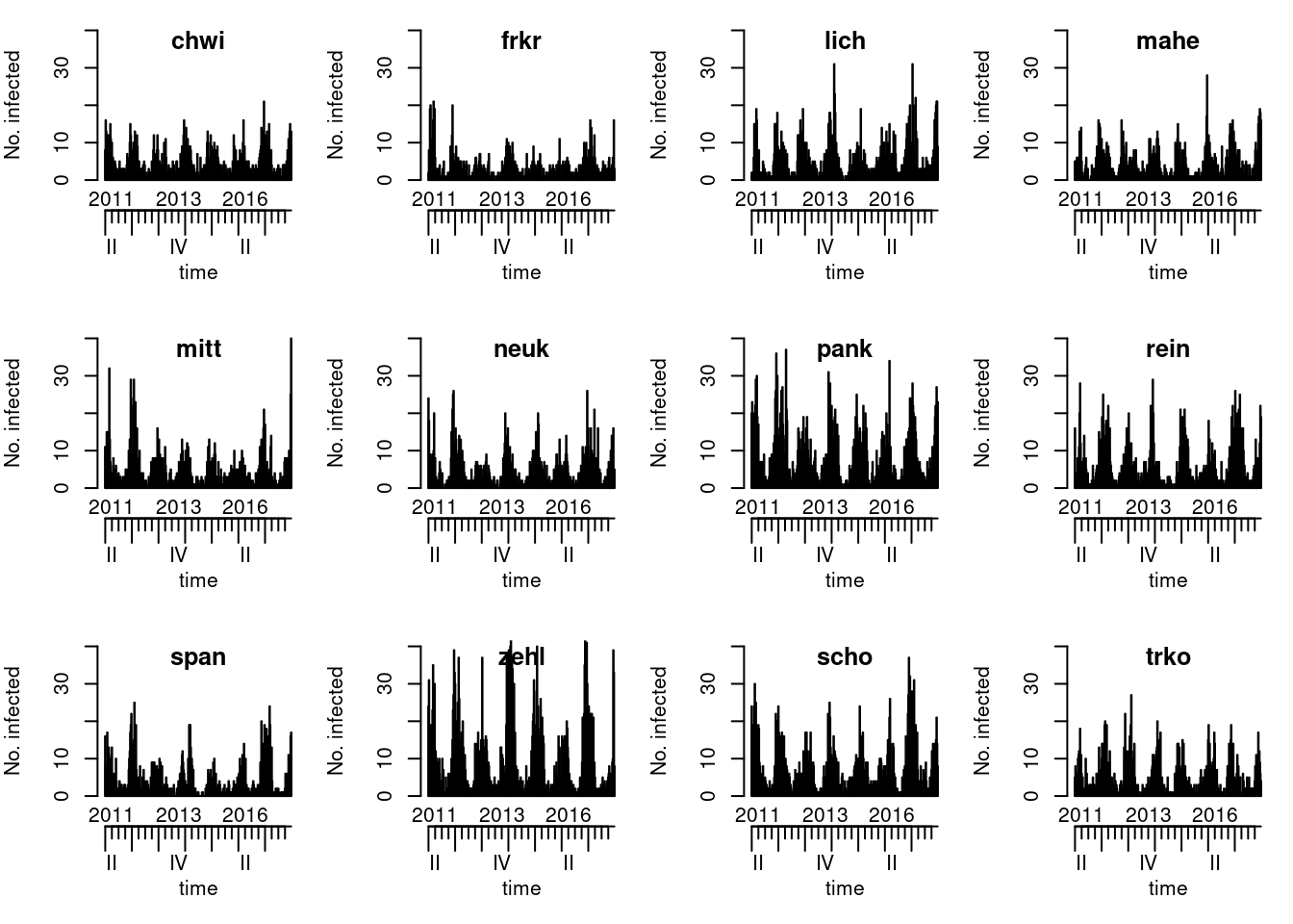
Exploring the data
Start by exploring the temporal and spatial distribution of
the data. You can find different plotting options in
?plot.sts.
Solution
# map:
# as population(noroBE) contains population fractions rather than raw
# population sizes setting population = 100000/<population of Berlin>
# will yield cumulative incidence per 100.000 inhabitants; see ?stsplot_space
plot(noroBE, observed ~ unit, population = 100000/3500000, labels = TRUE)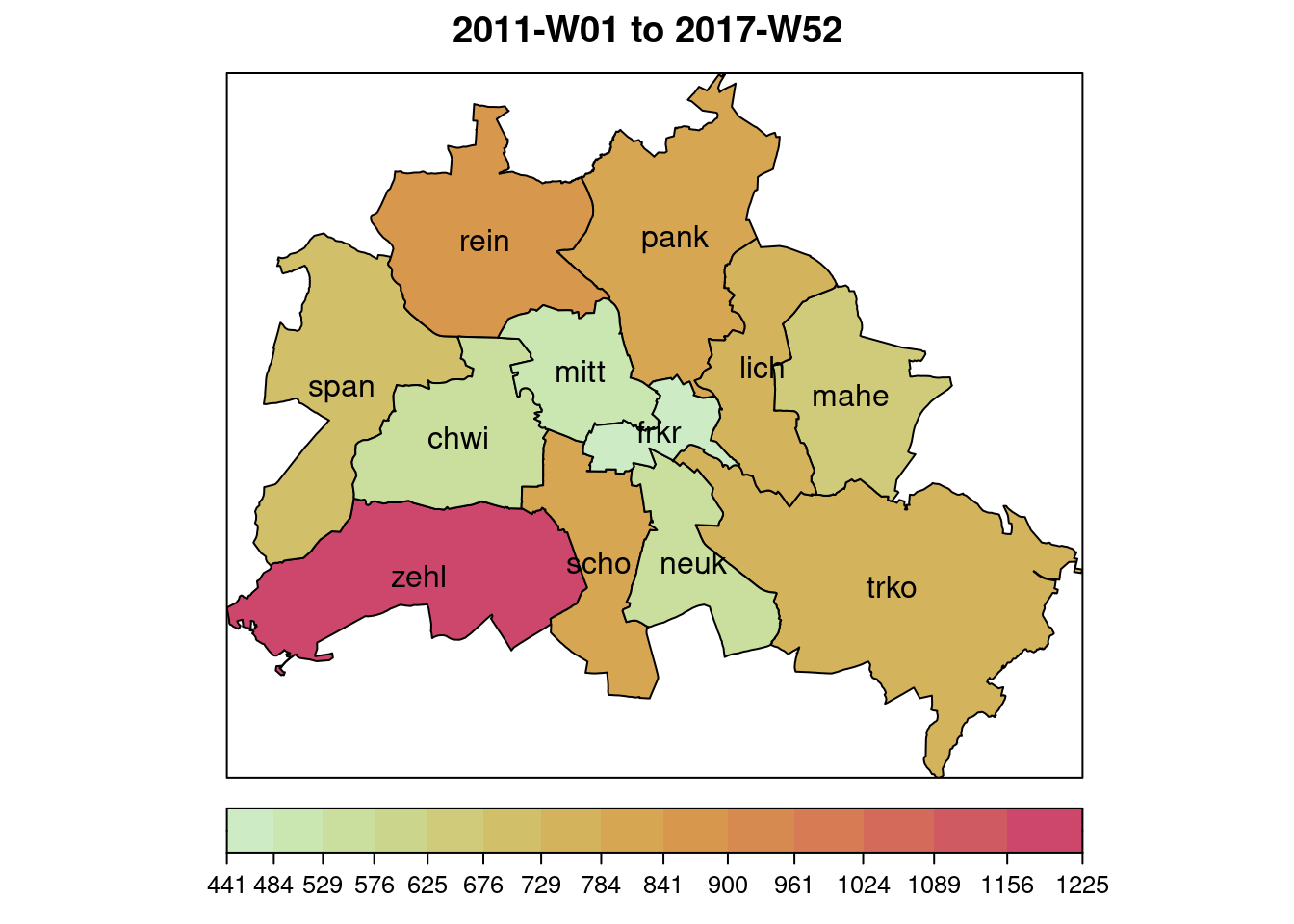
We moreover take a look at the slots
populationFrac (population fraction) and
neighbourhood of the sts object. The
latter contains path distances between the districts: e.g.,
chwi and frkr have a distance of 2 as you need
to go through mitt or scho. These distances
will later be relevant for spatial coupling.
Give me a hint on where to find these
You can list the contents of ansts object using
str(). Note that as we are dealing with an S4 object, it has slots, which
can be accessed using @ rather than $.
Solution
          chwi       frkr      lich       mahe       mitt       neuk      pank       rein
[1,] 0.0923389 0.07839664 0.0755159 0.07226963 0.09709093 0.09083884 0.1073534 0.06971871
[2,] 0.0923389 0.07839664 0.0755159 0.07226963 0.09709093 0.09083884 0.1073534 0.06971871
[3,] 0.0923389 0.07839664 0.0755159 0.07226963 0.09709093 0.09083884 0.1073534 0.06971871
[4,] 0.0923389 0.07839664 0.0755159 0.07226963 0.09709093 0.09083884 0.1073534 0.06971871
[5,] 0.0923389 0.07839664 0.0755159 0.07226963 0.09709093 0.09083884 0.1073534 0.06971871
[6,] 0.0923389 0.07839664 0.0755159 0.07226963 0.09709093 0.09083884 0.1073534 0.06971871
           span       zehl       scho      trko
[1,] 0.06537046 0.08505422 0.09617513 0.0698772
[2,] 0.06537046 0.08505422 0.09617513 0.0698772
[3,] 0.06537046 0.08505422 0.09617513 0.0698772
[4,] 0.06537046 0.08505422 0.09617513 0.0698772
[5,] 0.06537046 0.08505422 0.09617513 0.0698772
[6,] 0.06537046 0.08505422 0.09617513 0.0698772
# note: this is a matrix as in principle the population faction could vary over time.
# neighbourhood structure:
noroBE@neighbourhood # neighbourhood(noroBE) does the same chwi frkr lich mahe mitt neuk pank rein span zehl scho trko
chwi 0 2 3 4 1 2 2 1 1 1 1 3
frkr 2 0 1 2 1 1 1 2 3 2 1 1
lich 3 1 0 1 2 2 1 2 3 3 2 1
mahe 4 2 1 0 3 2 2 3 4 4 3 1
mitt 1 1 2 3 0 2 1 1 2 2 1 2
neuk 2 1 2 2 2 0 2 3 3 2 1 1
pank 2 1 1 2 1 2 0 1 2 3 2 2
rein 1 2 2 3 1 3 1 0 1 2 2 3
span 1 3 3 4 2 3 2 1 0 1 2 4
zehl 1 2 3 4 2 2 3 2 1 0 1 3
scho 1 1 2 3 1 1 2 2 2 1 0 2
trko 3 1 1 1 2 1 2 3 4 3 2 0Developing a multivariate model step by step
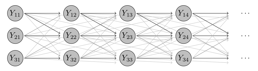
Step 1: Seasonality in the endemic component, all parameters shared, no coupling.
We start by a very simple model where for districts \(i = 1, \dots, K\) we assume \[\begin{align} Y_{it} \ \mid \ \ \text{past} & \sim \text{NegBin}(\mu_{it}, \psi)\\ \mu_{it} & = \nu_t + \lambda Y_{i, t - 1} \end{align}\] and \[ \nu_{t} = \alpha^\nu + \beta^\nu \sin(2\pi t/52) + \gamma^\nu \cos(2\pi t/52). \] This model features neither region-speciic parameters nor spatial coupling. To get you started the code for this model is provided. In the following steps you’ll be able to extend upon this basic formulation.
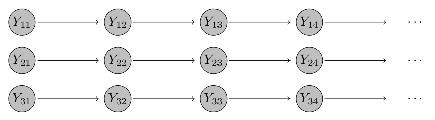
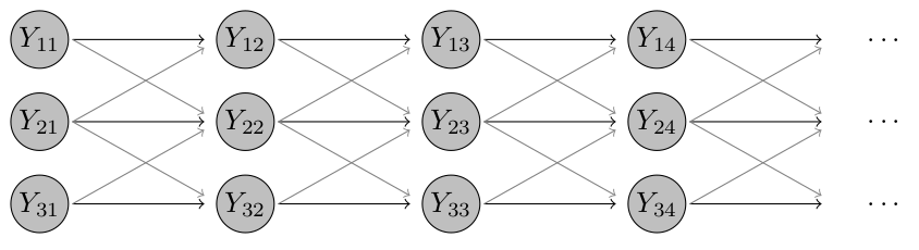
Click for an intuitive visual sketch of this model
In a setting with just \(K = 3\) districts the model could be illustrated as follows – case numbers the different districts are independent and only depend on the previous value in the same district.
Code:
# first define a subset of the data to which to fit (will be used in all model
# fits to ensure comparability of AIC values):
subset_fit <- 6:(nrow(noroBE@observed) - 52)
# we are leaving out the last year and the first 5 observations
# the latter serves to ensure comparability models with
# higher-order lags, see below.

##################################################################
# Model 1:
# control list:
ctrl1 <- list(end = list(f = addSeason2formula(~1, S = 1)), # seasonality in end
              # S = 1 means one pair of sine / cosine waves is included
              ar = list(f = ~ 1), # no seasonality in ar
              family = "NegBin1", # negative binomial (rather than Poisson)
              subset = subset_fit)
# fit model
fit1 <- hhh4(noroBE, ctrl1)
To inspect the model fit you can check out its summary
and some plots (check ?plot.hhh4 for options).
Solution
Call:
hhh4(stsObj = noroBE, control = ctrl1)

Coefficients:
                        Estimate  Std. Error
ar.1                    -0.72854   0.03453
end.1                    0.84477   0.02860
end.sin(2 * pi * t/52)   0.09024   0.02806
end.cos(2 * pi * t/52)   0.88574   0.02856
overdisp                 0.22957   0.01076

Log-likelihood:   -8780.82
AIC:              17571.64
BIC:              17602.7

Number of units:        12
Number of time points:  307
# you can set idx2Exp = TRUE to get all estimates on the exp-transformed scale
summary(fit1, idx2Exp = TRUE)
Call:
hhh4(stsObj = noroBE, control = ctrl1)

Coefficients:
                             Estimate  Std. Error
exp(ar.1)                    0.48261   0.01667
exp(end.1)                   2.32745   0.06657
exp(end.sin(2 * pi * t/52))  1.09443   0.03071
exp(end.cos(2 * pi * t/52))  2.42477   0.06925
overdisp                     0.22957   0.01076

Log-likelihood:   -8780.82
AIC:              17571.64
BIC:              17602.7

Number of units:        12
Number of time points: 307 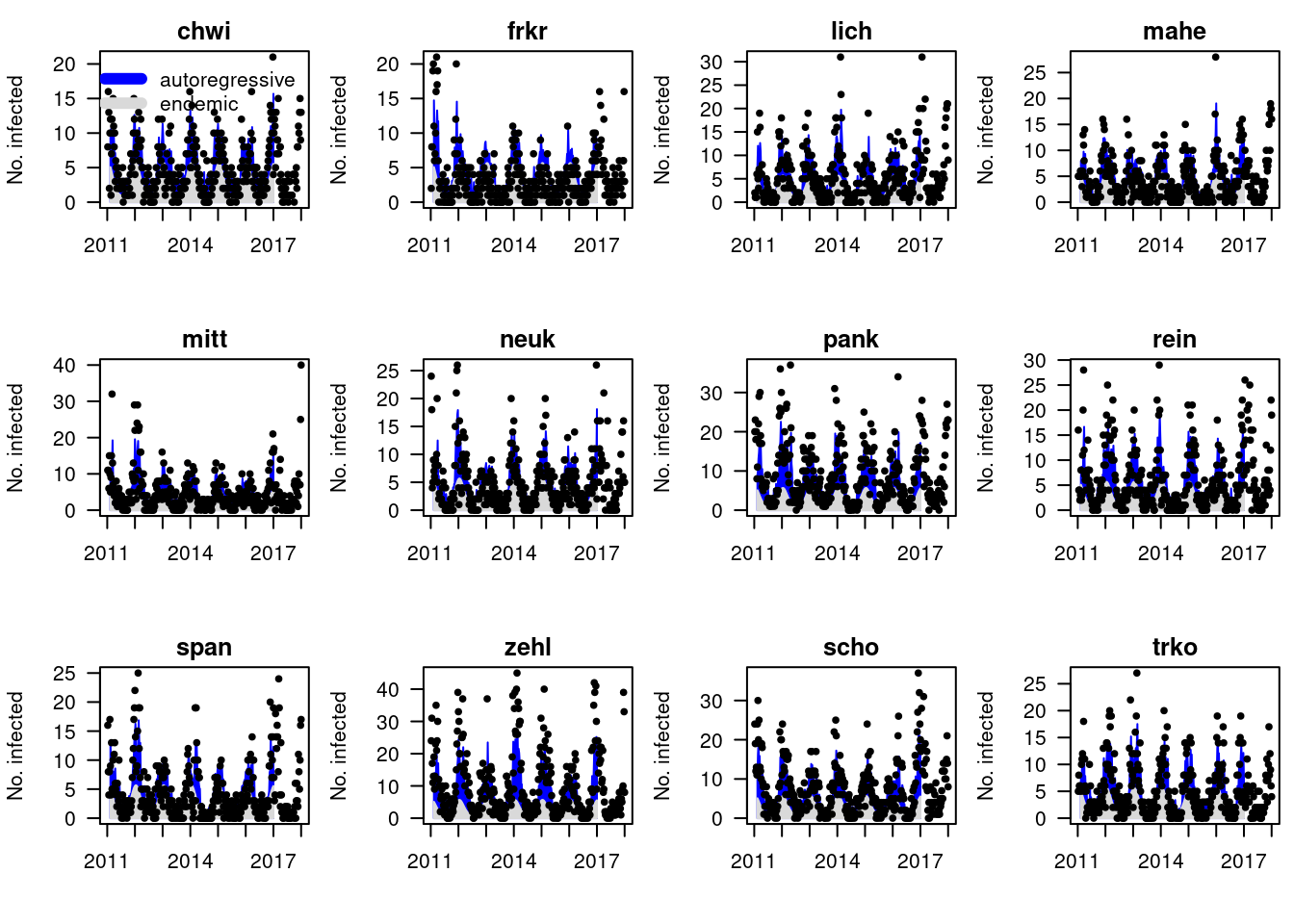
[1] 17571.64For model inspection I like looking at Pearson residuals \[ \frac{Y_{it} - \hat{\mu}_{it}}{\hat{\sigma}_{it}} = \frac{Y_{it} - \hat{\mu}_{it}}{\sqrt{\hat{\mu}_{it} + \hat{\mu}_{it}^2/\psi}}. \] In a well-specified model, the Pearson residuals should have roughly mean 0, standard deviation 1 and no autocorrelation.
residuals() with type = "pearson" are
currently only available in the
development version of surveillance (not needed)
which you might be able to install via (untested)
but you can instead use the following little auxiliary function:
# helper function to compute Pearson residuals. Just provide the model fit
# as the only argument.
# returns a matrix with Pearson residuals in the different strata (columns)
# and time points (rows)
# note: this is a bit more complicated as it also handles an extended version
# of the hhh4 class called hhh4lag
pearson_residuals <- function(hhh4Obj){
  # compute raw residuals:
  response_residuals <- residuals(hhh4Obj, type = "response")
  # compute standard deviations:
  if(inherits(hhh4Obj, "hhh4lag")){
    sds <- sqrt(fitted(hhh4Obj) +
                  fitted(hhh4Obj)^2/hhh4addon:::psi2size.hhh4lag(hhh4Obj))
  }else{
    sds <- sqrt(fitted(hhh4Obj) +
                  fitted(hhh4Obj)^2/surveillance:::psi2size.hhh4(hhh4Obj))
  }
  # compute Pearson residuals:
  pearson_residuals <- response_residuals/sds
  return(pearson_residuals)
}
On a side note: surveillancedoes support deviance
residuals, which serve a similar purpose, see
?residuals.hhh4.
Compute some region-wise summary statistics of Pearson residuals to get an idea of the shortcomings of this model.
Solution
pr1 <- pearson_residuals(fit1)
# deviance residuals as implemented in the package
# serve a similar purpose and are quite similar
# for large count values.
# dr1 <- residuals(fit1, type = "deviance")


# compute district-wise means and standard deviations:
colMeans(pr1)
chwi frkr lich mahe mitt neuk pank
-0.040128818 -0.354497174 -0.026596771 -0.149654100 -0.098957012 -0.139634691 0.363677331
rein span zehl scho trko
-0.006394507 -0.203281407 0.422776136 0.208763434 -0.023204469 chwi frkr lich mahe mitt neuk pank rein span
0.8969573 0.8394516 0.9984702 0.9348625 0.9594755 0.8998828 1.1386447 0.9955265 0.9606598
zehl scho trko
1.2538557 1.0589218 0.9730101 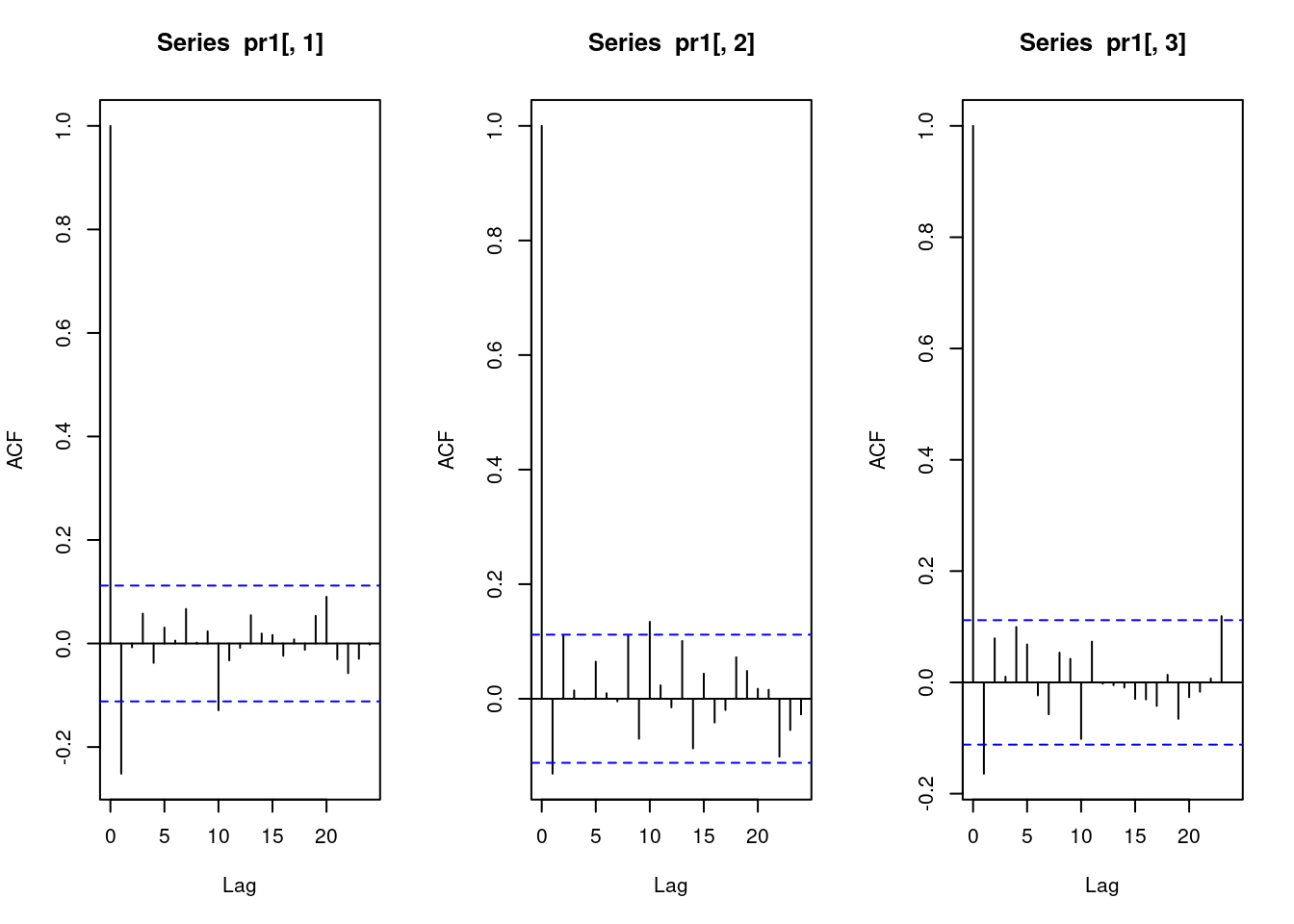
In each district, the Pearson residuals should have mean and standard deviations of approximately 0 and 1, respectively, which is clearly not the case. By sharing all parameters, fitted values are systematically larger than observed in some districts and smaller in others.
Moreover, in a correctly specified model, the Pearson residuals would be uncorrelated, which is clearly not the case either.Step 2: Adding district-specific parameters.
As the districts are of different sizes and have different incidence levels, we include district-specific parameters and extend the model to \[\begin{align} Y_{it} \ \mid \ \ \text{past} & \sim \text{NegBin}(\mu_{it}, \psi)\\ \mu_{it} & = \nu_{it} + \lambda_i Y_{i, t - 1}\\ \nu_{it} & = \alpha^\nu_i + \beta^\nu \sin(2\pi t/52) + \gamma^\nu \cos(2\pi t/52) \end{align}\] Note that the parameters for seasonality are still shared (though you can try out district-specific ones).
Try to fit this model to the data. You can check out
?fe on district-specific parameters.
Solution
##################################################################
# Model 2:
# We use fe(..., unitSpecific = TRUE) to add fixed effects for each unit,
# in this case intercepts (1). Seasonality parameters are still shared
# across districts
ctrl2 <- list(end = list(f = addSeason2formula(~0 + fe(1, unitSpecific = TRUE),
                                               S = 1)),
              ar = list(f = ~ 0 + fe(1, unitSpecific = TRUE)),
              family = "NegBin1",
              subset = subset_fit)
# Note: ~0 is necessary as otherwise one would (implicitly) add two intercepts
# unit-specific dispersion parameters could be added by setting family = "NegBinM"
fit2 <- hhh4(noroBE, ctrl2)
# check parameter estimates:
summary(fit2)
Call:
hhh4(stsObj = noroBE, control = ctrl2)

Coefficients:
                        Estimate   Std. Error
ar.1.chwi               -1.795086   0.402460
ar.1.frkr               -1.259748   0.182296
ar.1.lich               -1.087080   0.177651
ar.1.mahe               -0.957952   0.145501
ar.1.mitt               -1.335034   0.214060
ar.1.neuk               -0.967629   0.159855
ar.1.pank               -0.753360   0.129017
ar.1.rein               -0.668191   0.103620
ar.1.span               -0.823339   0.125950
ar.1.zehl               -0.659794   0.095464
ar.1.scho               -0.865145   0.132413
ar.1.trko               -1.002428   0.165175
end.sin(2 * pi * t/52)   0.121489   0.024384
end.cos(2 * pi * t/52)   0.923900   0.024745
end.1.chwi               1.181472   0.088438
end.1.frkr               0.604251   0.081671
end.1.lich               1.020524   0.089385
end.1.mahe               0.791906   0.089509
end.1.mitt               1.010631   0.081603
end.1.neuk               0.823126   0.097049
end.1.pank               1.298509   0.104632
end.1.rein               0.791816   0.097056
end.1.span               0.648208   0.092789
end.1.zehl               1.297808   0.091415
end.1.scho               1.189950   0.093128
end.1.trko               0.997664   0.094204
overdisp                 0.197678   0.009884

Log-likelihood:   -8655.46
AIC:              17364.92
BIC:              17532.63

Number of units:        12
Number of time points: 307 [1] 17364.92Next, let’s again again check the Pearson residuals.
Solution
# compute Pearson residuals and check their mean and variance:
pr2 <- pearson_residuals(fit2)
colMeans(pr2)
chwi frkr lich mahe mitt neuk pank
0.020061368 0.025144794 -0.010413219 0.003481020 -0.004801394 -0.006139166 -0.012998766
rein span zehl scho trko
-0.004079849 -0.001710578 -0.022435249 -0.007614639 -0.016314666 chwi frkr lich mahe mitt neuk pank rein span
0.8969573 0.8394516 0.9984702 0.9348625 0.9594755 0.8998828 1.1386447 0.9955265 0.9606598
zehl scho trko
1.2538557 1.0589218 0.9730101 Note that we could also add district-specific dispersion parameters
\(\psi_i\) by setting
family = "NegBinM", but for simplicity we stick with the
shared overdispersion parameter.
Step 3: Adding dependence between districts.
For now we have been modelling each district separately (while
sharing some parameters). We now add dependencies via the
ne (neighbourhood) component. The simplest version is a
model where only direct neighbours affect each other, \[\begin{align}
Y_{it} \ \mid \ \ \text{past} & \sim \text{NegBin}(\mu_{it}, \psi)\\
\mu_{it} & = \nu_{it} + \lambda_i Y_{i, t - 1} + \phi_i \sum_{j \sim
i} w_{ji} Y_{j, t - 1}.
\end{align}\] Here, the relationship \(\sim\) indicates direct neighbourhood. The
weights \(w_{ji}\) can be chosen in two
ways.
- if
normalize == TRUE: \(w_{ji} = 1/\) (number of neighbours of \(j\)) if \(i \sim j\), 0 else - if
normalize == FALSE: \(w_{ji} = 1\) if \(i \sim j\), 0 else
We usually use normalize = TRUE, which is based on the
intuition that each district splits up its infectious pressure equally
among its neighbours. Note that in this formulation, the autoregression
on past incidence from the same district and others are handled each on
their own with separate parameters.
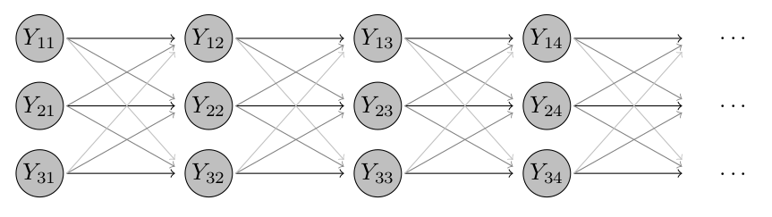
Click for an intuitive visual sketch of this model
In our example with just three districts, where district 2 is neighbouring both 1 and 3, but 1 and 3 are not neighbours, the model looks as follows. The grey lines indicate that these dependencies are typically weaker than the ones to previous values from the same district.
As documented in ?hhh4, the neighbourhood weights \(w_{ji}\) are obtained from the matrix
noroBE@nighborhood via
noroBE@neighbourhood == 1. You can convince yourself up here that in the encoding used for the path
distances, 1 indeed indicates direct neighbourhood. All
other entries will be treated equally as “non-neighbours”.
Try to add an ne component to your model by
modifying the control list or by using update. You
can check out ?hhh4 for details.
Solution
# The default setting for the ne component is to use weights
# neighbourhood(stsObj) == 1 (see ?hhh4).
neighbourhood(noroBE) == 1
chwi frkr lich mahe mitt neuk pank rein span zehl scho trko
chwi FALSE FALSE FALSE FALSE TRUE FALSE FALSE TRUE TRUE TRUE TRUE FALSE
frkr FALSE FALSE TRUE FALSE TRUE TRUE TRUE FALSE FALSE FALSE TRUE TRUE
lich FALSE TRUE FALSE TRUE FALSE FALSE TRUE FALSE FALSE FALSE FALSE TRUE
mahe FALSE FALSE TRUE FALSE FALSE FALSE FALSE FALSE FALSE FALSE FALSE TRUE
mitt TRUE TRUE FALSE FALSE FALSE FALSE TRUE TRUE FALSE FALSE TRUE FALSE
neuk FALSE TRUE FALSE FALSE FALSE FALSE FALSE FALSE FALSE FALSE TRUE TRUE
pank FALSE TRUE TRUE FALSE TRUE FALSE FALSE TRUE FALSE FALSE FALSE FALSE
rein TRUE FALSE FALSE FALSE TRUE FALSE TRUE FALSE TRUE FALSE FALSE FALSE
span TRUE FALSE FALSE FALSE FALSE FALSE FALSE TRUE FALSE TRUE FALSE FALSE
zehl TRUE FALSE FALSE FALSE FALSE FALSE FALSE FALSE TRUE FALSE TRUE FALSE
scho TRUE TRUE FALSE FALSE TRUE TRUE FALSE FALSE FALSE TRUE FALSE FALSE
trko FALSE TRUE TRUE TRUE FALSE TRUE FALSE FALSE FALSE FALSE FALSE FALSE# this is because historically neighbourhood matrices were just binary
# however, the path distances are coded in a way that direct neighbours have
# distance 1, meaning that there is no need to modify the neighbourhood matrix
##################################################################
# Model 3:
ctrl3 <- list(end = list(f = addSeason2formula(~0 + fe(1, unitSpecific = TRUE),
S = 1)),
ar = list(f = ~ 0 + fe(1, unitSpecific = TRUE)),
ne = list(f = ~ 0 + fe(1, unitSpecific = TRUE), normalize = TRUE),
# now added ne component to reflect cross-district dependencies
family = "NegBin1",
subset = subset_fit)
# normalize = TRUE normalizes weights by the number of neighbours of the
# exporting district
fit3 <- hhh4(noroBE, ctrl3)
AIC(fit3)[1] 17271.12# alternative: use update
# fit3 <- update(fit2, ne = list(f = ~ 0 + fe(1, unitSpecific = TRUE),
# weights = neighbourhood(noroBE) == 1, # little bug?
# normalize = TRUE))
summary(fit3) # parameters for different districts are quite different
Call:
hhh4(stsObj = noroBE, control = ctrl3)

Coefficients:
                        Estimate   Std. Error
ar.1.chwi               -2.984424   1.350606
ar.1.frkr               -1.546018   0.255272
ar.1.lich               -1.481704   0.269704
ar.1.mahe               -1.042180   0.165513
ar.1.mitt               -1.684145   0.325195
ar.1.neuk               -1.178880   0.203516
ar.1.pank               -0.950771   0.162474
ar.1.rein               -0.739190   0.113666
ar.1.span               -1.030189   0.159685
ar.1.zehl               -0.700978   0.109133
ar.1.scho               -1.140107   0.188365
ar.1.trko               -0.954548   0.156077
ne.1.chwi               -1.556838   0.229854
ne.1.frkr               -2.105432   0.303360
ne.1.lich               -1.333358   0.275089
ne.1.mahe               -2.082596   1.001100
ne.1.mitt               -1.382118   0.285452
ne.1.neuk               -1.005697   0.308230
ne.1.pank               -0.594043   0.265078
ne.1.rein               -1.531222   0.365439
ne.1.span               -1.496264   0.237766
ne.1.zehl               -1.197674   0.519991
ne.1.scho               -1.174415   0.268474
ne.1.trko               -2.805666   1.088384
end.sin(2 * pi * t/52)   0.013954   0.037300
end.cos(2 * pi * t/52)   0.918633   0.033880
end.1.chwi               0.817175   0.143907
end.1.frkr               0.142450   0.200990
end.1.lich               0.636253   0.176280
end.1.mahe               0.715465   0.135111
end.1.mitt               0.541823   0.187192
end.1.neuk               0.444922   0.175794
end.1.pank               0.867238   0.188664
end.1.rein               0.349285   0.222273
end.1.span               0.143326   0.183118
end.1.zehl               1.068714   0.140279
end.1.scho               0.730291   0.182337
end.1.trko               0.866186   0.143240
overdisp                 0.182920   0.009464

Log-likelihood:   -8596.56
AIC:              17271.12
BIC:              17513.37

Number of units:        12
Number of time points: 307 [1] 17271.12You can explore the importance of the neighbourhood component by re-plotting the model fits.
Solution
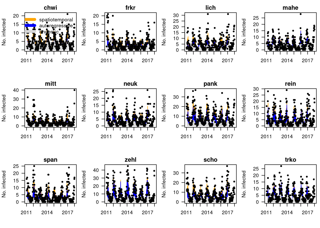 Plotting the model fits, we see that for certain districts the
neighbourhood component is very important (
Plotting the model fits, we see that for certain districts the
neighbourhood component is very important (chwi), for
others negligible (trko). This may be due to poor
identifiability (often the autoregressive terms from the same and other
districts are strongly correlated).
Step 4: Using a power law for spatial dependence.
The above formulation requires a lot of parameters as the autoregressions on the same and other regions are handled separately. Moreover, it only takes into account direct neighbours. A more parsimonious model also allowing for dependencies between indirect neighbours is a power-law formulation, where we set \[\begin{align} \mu_{it} & = \nu_{it} + \lambda_i Y_{i, t - 1} + \phi_i \sum_{j = 1}^K w_{ji} Y_{j, t - 1} \end{align}\] with weights \(w_{ji}\) defined as follows.
- if
normalize == FALSE: \[ w_{ji} = (o_{ji} + 1)^{-\rho} \]. - if
normalize == TRUE: \[ w_{ji} = \frac{(o_{ji} + 1)^{-\rho}}{\sum_{i = 1}^K (o_{jk} + 1)^{-\rho}}$ \] Here, \(o_{ji}\) is the path distance between districts \(j\) and \(i\), i.e., the entries ofnoroBE@neihbourhood.
Click for an intuitive visual sketch of this model
Returning to our simple illustration with three districts, this step adds some additional connections between indirect neighbours (districts 1 and 3). They are shown in light grey as by construction of the model they are weaker than those between neighbouring districts.
Try to add a power law with normalization to the model (see
?W_powerlaw).
Some hints
- If you want to fit the model as described above, your control list
should no longer contain an
arelement. - The
maxlagargument does not play much of a role in this toy examples, you can e.g., set it to 5.
Solution
##################################################################
# Model 4
# For the next model version we will formally include the autoregressive into
# the neighbourhood component
# (i.e. do no longer treat autoregression on the same district separately).
# This can be done as follows.
# First we need to adapt the neighbourhood matrix, shifting by one
noroBE_power <- noroBE
noroBE_power@neighbourhood <- noroBE@neighbourhood + 1
# new control argument:
ctrl4 <- list(end = list(f = addSeason2formula(~0 + fe(1, unitSpecific = TRUE),
S = 1)),
# note: line ar = ... is removed
ne = list(f = ~0 + fe(1, unitSpecific = TRUE),
weights = W_powerlaw(maxlag=5, normalize = TRUE,
log = TRUE)), # this is new
family = "NegBin1",
subset = subset_fit)
# normalize = TRUE normalizes weights by the number of neighbours of the
# exporting district
# log = TRUE means optimization will be done on a log scale, ensuring
# positivity of the decay parameter (which is desirable)
fit4 <- hhh4(noroBE_power, ctrl4)
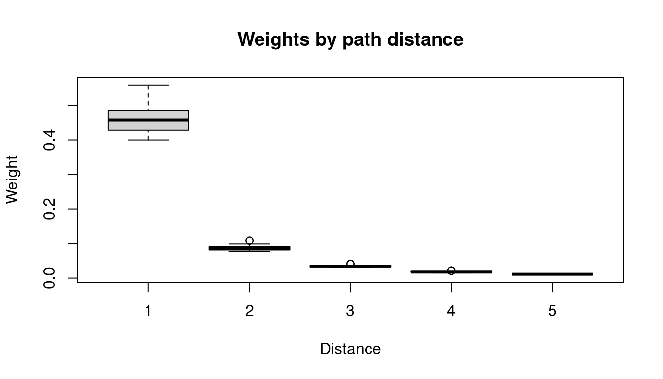
AIC(fit4)[1] 17233.06We can visualize the weights \(w_{ji}\) as a function of the path
dependence \(o_{ji}\) (see
?plot.hhh4).
Step 5: Adding seasonality to the epidemic component.
Including seasonality in the ar and ne
components when both are present can lead to identifiability issues. In
the more parsimonious model where only the ne component is
present, however, including seasonal terms here can considerably improve
the model fit. Extend the previous model to include seasonal
terms (with S = 1) in the
necomponent.
Solution
##################################################################
# Model 5:
ctrl5 <- list(end = list(f = addSeason2formula(~0 + fe(1, unitSpecific = TRUE),
                                               S = 1)),
              # now adding seasonality to the ne component:
              ne = list(f =  addSeason2formula(~0 + fe(1, unitSpecific = TRUE),
                                               S = 1),
                        weights = W_powerlaw(maxlag=5, normalize = TRUE,
                                             log=TRUE)), # this is new
              family = "NegBin1",
              subset = subset_fit)
fit5 <- hhh4(noroBE_power, ctrl5)
AIC(fit5)
[1] 17205.41Bonus steps
If you have made it until here before the session is over – congratulations! Below you will find some additional ideas to keep you busy. They do not have a specific ordering and you can try them out independently of each other.
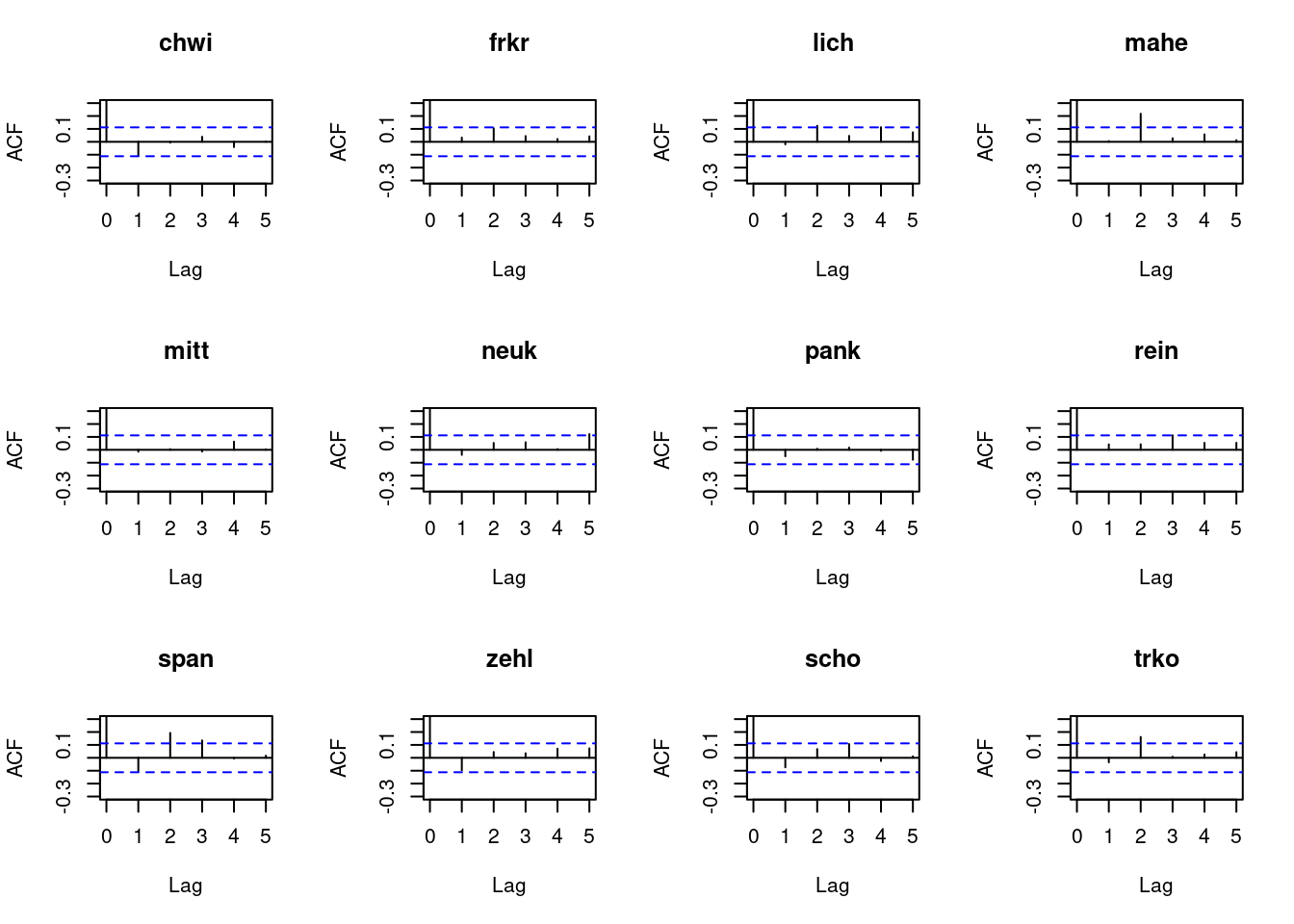
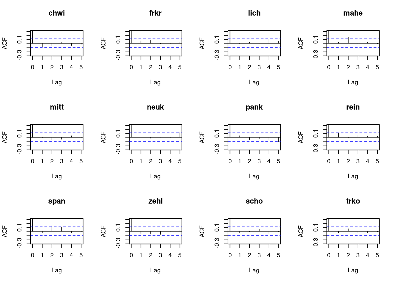
Bonus: Adding higher-order lags.
Let us re-consider the autocorrelation of the Pearson residuals. You will see that for several regions there are pronounced residual autocorrelations at lags 2 or 3, indicating that there is additional information to be exploited.
Solution
# compute Pearson residuals:
pr5 <- pearson_residuals(fit4)
par(mfrow = c(3, 4))
for(unit in colnames(pr5)){
  acf(pr5[, unit], lag.max = 5, ylim = c(-0.3, 0.3), main = unit)
}
To remedy this, higher-order lags can be included in the model. This
functionality is implemented in the hhh4addon
package. For technical reasons this package is not on CRAN, but you
can install it from GitHub.
## to install hhh4addon:
# install.packages("remotes")
# remotes::install_github("jbracher/hhh4addon", build_vignettes = TRUE)

library(hhh4addon)
Registered S3 methods overwritten by 'hhh4addon':
method from
confint.oneStepAhead surveillance
plot.oneStepAhead surveillance
quantile.oneStepAhead surveillanceThis is a development version of hhh4addon. It modifies and extends functionalities of surveillance:hhh4.
Attache Paket: 'hhh4addon'Das folgende Objekt ist maskiert 'package:surveillance':
decompose.hhh4The model then becomes
\[ \mu_{it} = \nu_{it} + \lambda_i Y_{i, t - 1} + \phi_i \sum_{j = 1}^K \sum_{d = 1}^D u_d w_{ji} Y_{j, t - 1}. \]
Lag weights are (usually) governed by a single parameter, which is
fed into a function returning the weights. The package contains the
several parsimonious parameterizations (?profile_par_lag),
e.g.,:
- geometric: \(\tilde{u}_d = \alpha(1 - \alpha)^{d - 1}\)
- Poisson: \(\tilde{u}_d = \alpha^{d - 1}\exp(-\alpha)/(d - 1)!\)
The lag weights are standardized so they sum up to one, setting \(u_d = \tilde{u}_d / \sum_{i = 1}^D \tilde{u}_{i}\). In mechanistic interpretation, they correspond to the generation time / serial interval distribution.
Click for an intuitive visual sketch of this model
Returning a last time to our toy illustration of three districts, this step adds a whole lot of (typically weak) connections between non-neighbouring time points.
Try to fit a model with geometric lag weights (the default)
using the function profile_par_lag. Then re-check the
Pearson residuals.
Why does this function have such a strange name?
Orininally there was afunctionhhh4lag which allowed for
lag weights specified by the user and typically based on literature
estimates of the generation time distribution. Functionality to estimate
the a weighting parameter \(\alpha\)
was only added later and is based on a profile
likelihood approach. As this parameter is called
par_lag in the implementation, the function running profile
likelihood inference is called profile_par_lag.
Solution
##################################################################
# Model 7
ctrl7 <- list(end = list(f = addSeason2formula(~0 + fe(1, unitSpecific = TRUE),
                                               S = 1)),
              # note: line ar = ... is removed
              ne = list(f = addSeason2formula(~0 + fe(1, unitSpecific = TRUE),
                                              S = 1),
                        weights = W_powerlaw(maxlag=5, normalize = TRUE,
                                             log=TRUE)), # this is new
              family = "NegBin1",
              subset = subset_fit,
              # (no specification of par_lag in the control)
              funct_lag = geometric_lag)
# now use profile_par_lag (applies a profile likelihood procedure to estimate
# the lag decay parameter)
fit7 <- profile_par_lag(noroBE_power, ctrl7)
AIC(fit7)
[1] 17138.12We can plot the weights as estimated from the data:
# plot the weights assigned to the different lags:
par(mfrow = 1:2)
plot(fit7$distr_lag, type = "h", xlab = "lag",
ylab = "weight", ylim = 0:1)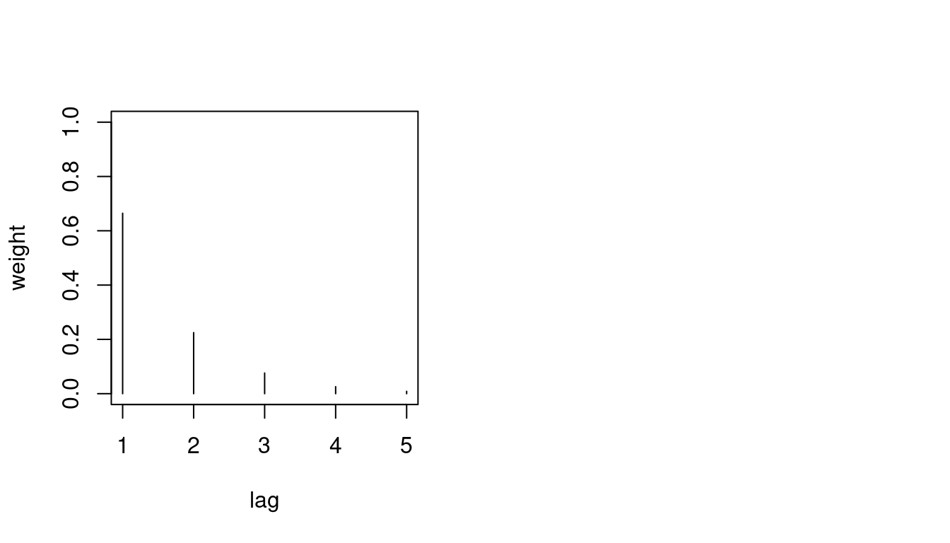 And consider the Pearson residuals, which look less problematic than
before.
And consider the Pearson residuals, which look less problematic than
before.
# check Pearson residuals
pr7 <- pearson_residuals(fit7)
par(mfrow = c(3, 4))
for(unit in colnames(pr7)){
  acf(pr7[, unit], lag.max = 5, ylim = c(-0.3, 0.3), main = unit)
}
Bonus: One-step-ahead forecasting.
The packages contain functionality to imitate one-step-ahead
(out-of-sample) forecasts retrospectively. To this end, the model is
sequentially re-fitted, always including all data up to a given week.
Then a one-week-ahead plug-in prediciton is obtained for the next week.
We apply this to obtain predictions for weeks 313 through 364 which we
had excluded from model fitting so far. Subsequently, you can use
scores to evaluate the one-step-ahead predictions using
several different scoring rules. We
compute the following:
- the logarithmic score, also called negative predictive log-likelihood (informal explanation: this reflects how likely the observed outcomes were under your predictions)
- the CRPS (informal explanation: this describes “how far” the observations were from the predictions you issued)
For both lower values are better.
As this may be a bit tedious to piece together I am providing
the analysis for fit2 and fit4 and you can
explore things based on this skeleton.
Find the code here
##################################################################
# one-step-ahead forecasting: generate forecasts sequentially
# compare models 2, 4 and 7
log2 <- capture.output(owa2 <- oneStepAhead(fit2, tp = c(312, 363)))
log4 <- capture.output(owa4 <- oneStepAhead(fit4, tp = c(312, 363)))
rm(log2, log4)
# the weird capture.output fourmulation is needed to suppress
# numerous cat() messages.
# you could also just use
# owa2 <- oneStepAhead(fit2, tp = c(312, 363))
owa7 <- oneStepAhead_hhh4lag(fit7, tp = c(312, 363))
Lag weights are not re-estimated for the one-step-ahead forecasts (set refit_par_lag = TRUE to re-fit them). chwi frkr lich mahe mitt neuk pank rein span zehl
313 10.143891 5.997015 8.315079 7.550797 12.276675 9.072281 18.06990 12.35556 13.161304 20.62583
314 10.052363 6.133326 9.568715 7.025105 12.332588 11.455435 20.52966 10.66938 10.103430 23.18901
315 10.837812 6.638302 10.085745 8.250180 10.817444 10.246092 22.11388 17.05596 8.692397 24.61323
316 9.737658 6.614878 16.126879 8.251785 8.842089 8.346344 24.43109 14.89341 7.391036 19.24499
317 8.017484 5.761749 10.387913 6.531485 6.529512 7.030808 20.62327 11.56332 10.879236 19.91117
318 9.328702 7.435577 13.008535 6.949797 8.054874 9.280143 20.39342 11.20380 11.205468 19.68513
scho trko
313 19.19221 7.951694
314 18.21469 8.461257
315 21.20857 8.030405
316 17.81345 7.817094
317 14.02415 6.814946
318 16.13912 8.639782 chwi frkr lich mahe mitt neuk pank rein span zehl scho trko
313 10 4 10 5 17 16 23 5 7 24 17 5
314 12 8 9 10 6 8 23 26 3 24 28 3
315 11 7 31 7 3 5 28 14 4 14 18 2
316 5 8 6 5 0 5 22 8 18 20 12 4
317 13 16 20 6 7 11 20 8 14 17 18 6
318 7 8 7 5 3 16 9 20 12 22 31 11# plot one-step-ahead point forecasts:
plot(noroBE@observed[313:364, 1], pch = 20, xlab = "week", ylab = "value")
lines(owa2$pred[, 1], type = "l", col = 2)
lines(owa4$pred[, 1], type = "l", col = 4)
lines(owa7$pred[, 1], type = "l", col = 6)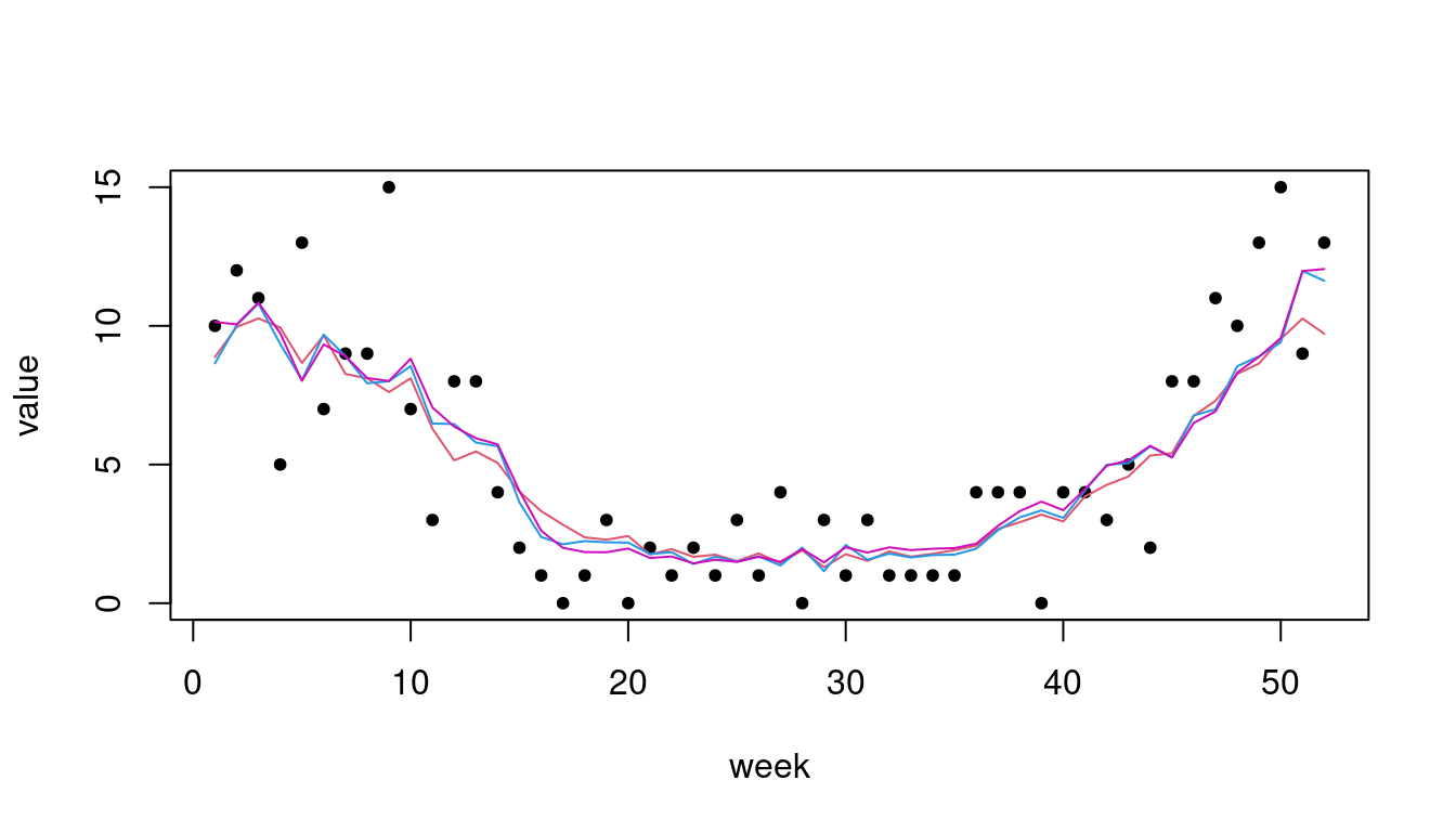
    logs      rps
2.506608 2.091024 logs rps
2.492431 2.066390 logs rps
2.475311 2.042008 We can see that the more complex model formulations also translate to
improved predictive performance (all scores being negatively oriented;
see ?scores).
Bonus: Including a covariate.
Norovirus transmission has been argued to depend on meteorological variables including temperature. We therefore uploaded a time series of weekly mean temperature values in Berlin (average of daily temperatures at 2pm, lagged by one week) in the data bundle for the workshop. These (or a transformation) can be used a a covariate.
data_temperature <- read.csv("data/temperature_berlin.csv")
temperature <- data_temperature$temperature7d
Try to include these in the model in a way you think might be helpful.
Find my minimal attempt here
I would assume temperature to modify the transmissibility of the
virus, so I included the covariate into the ar component of
a simple model.
# your formula could look as follows:
ctrl_temp <- list(end = list(f = addSeason2formula(~0 + fe(1, unitSpecific = TRUE),
                                              S = 1)),
             ar = list(f = ~ 0 + temperature + fe(1, unitSpecific = TRUE)),
             family = "NegBin1",
             subset = 6:312)


fit_temp <- hhh4(noroBE, ctrl_temp)
AIC(fit_temp)
[1] 17318.05[1] 17364.92fit2, which
is the same model just without the covariate. Up to you to check this in
more complex models.
Please keep in mind that this is a toy example to allow you to
explore the hhh4 framework, not a serious analysis of
norovirus epidemiology.