Tutorial 0: The data class
"sts"
Using ECDC data of monthly IMD counts
Template: sts.R
Abstract
If you’d like to come to grips with the dedicated data class
"sts" (surveillance time series) used as a basis
for the modelling and monitoring tools in the
surveillance package—maybe you intend to process your
own data—this tutorial is for you. It illustrates how to create an
"sts" object by importing public health surveillance data,
population numbers and a map. We will use data from the Surveillance Atlas of
Infectious Diseases of the European Centre for Disease Prevention
and Control (ECDC) on the monthly number of reported cases of
invasive meningococcal disease (IMD).
The code for the first section (import raw data) is provided in the R
script template sts.R that is part of the tutorials.zip
archive, which also contains the necessary data files. You can read the
description on this page, run the code, and then start with the
"sts" exercises in the subsequent sections.
Epidemiology of IMD (from Wikipedia)
It is spread through saliva and other respiratory secretions during coughing, sneezing, kissing, and chewing on toys. Inhalation of respiratory droplets from a carrier which may be someone who is themselves in the early stages of disease can transmit the bacteria. […] The incubation period is short, from 2 to 10 days.
Disclaimer (formally required by the ECDC)
The views and opinions of the authors expressed herein do not necessarily state or reflect those of the ECDC. The accuracy of the authors’ statistical analysis and the findings they report are not the responsibility of ECDC. ECDC is not responsible for conclusions or opinions drawn from the data provided. ECDC is not responsible for the correctness of the data and for data management, data merging and data collation after provision of the data. ECDC shall not be held liable for improper or incorrect use of the data.Caveat (about monthly counts)
The sole purpose of this exercise is to illustrate data import and the"sts" class. Note that monthly counts are
generally inconvenient for epidemic models (or timely monitoring, for
that matter) of IMD cases or common respiratory infections: a single
time interval would typically “hide” several generations of infections.
Import raw data (code provided)
We need to prepare the main ingredients of a spatial
"sts" object:
observedtime series of counts (by region)populationnumbers to calculate incidence valuesmapof the regions for visualizations
The bold words correspond to arguments of the sts()
constructor function.
observed time series of counts
The counts downloaded from the ECDC atlas cover the years 1999–2018 and are provided in a (gzip-compressed) CSV file. This is how the first 3 lines look like:
"HealthTopic","Population","Indicator","Unit","Time","RegionCode","RegionName","NumValue","TxtValue"
"Invasive meningococcal disease","Confirmed cases","Reported cases","N","1999-01","AT","Austria",11.000000000,""
"Invasive meningococcal disease","Confirmed cases","Reported cases","N","1999-01","BE","Belgium",24.000000000,""
The counts (NumValue) are given in the long format where
each row corresponds to one time/region combination. We import the
counts from the CSV file and reshape the data into the wide (matrix)
format with one column per region. This is the format typically used for
multivariate time series, including in sts()
and R’s basic ts()
function.
ecdc_long <- read.csv(
    file = "data/ECDC_surveillance_data_IMD.csv.gz",  # R can read compressed files
    na.strings = "-")  # always important to know how NA's are encoded!
head(ecdc_long, 10)
HealthTopic Population Indicator Unit Time RegionCode
1 Invasive meningococcal disease Confirmed cases Reported cases N 1999-01 AT
2 Invasive meningococcal disease Confirmed cases Reported cases N 1999-01 BE
3 Invasive meningococcal disease Confirmed cases Reported cases N 1999-01 CZ
4 Invasive meningococcal disease Confirmed cases Reported cases N 1999-01 DE
5 Invasive meningococcal disease Confirmed cases Reported cases N 1999-01 DK
6 Invasive meningococcal disease Confirmed cases Reported cases N 1999-01 EE
7 Invasive meningococcal disease Confirmed cases Reported cases N 1999-01 EL
8 Invasive meningococcal disease Confirmed cases Reported cases N 1999-01 ES
9 Invasive meningococcal disease Confirmed cases Reported cases N 1999-01 EU_EEA31
10 Invasive meningococcal disease Confirmed cases Reported cases N 1999-01 FI
RegionName NumValue TxtValue
1 Austria 11 NA
2 Belgium 24 NA
3 Czechia 5 NA
4 Germany 37 NA
5 Denmark 19 NA
6 Estonia 0 NA
7 Greece 18 NA
8 Spain 172 NA
9 EU/EEA 1020 NA
10 Finland 6 NA## exclude aggregate counts
ecdc_long <- subset(ecdc_long, !startsWith(RegionName, "EU"))
## reshape from long to wide format of multivariate time series
ecdc <- reshape(ecdc_long[c("Time", "RegionCode", "NumValue")],
direction = "wide", idvar = "Time", timevar = "RegionCode")
names(ecdc) <- sub("NumValue.", "", names(ecdc), fixed = TRUE)
row.names(ecdc) <- ecdc$Time; ecdc$Time <- NULL
head(ecdc) AT BE CZ DE DK EE EL ES FI FR IE IS IT LU MT NL NO PL SE SI UK LT PT LV HU SK CY BG RO
1999-01 11 24 5 37 19 0 18 172 6 43 53 2 36 0 0 81 4 11 2 1 495 NA NA NA NA NA NA NA NA
1999-02 14 37 8 48 17 0 16 123 9 65 43 2 31 0 2 68 11 9 3 0 267 NA NA NA NA NA NA NA NA
1999-03 12 49 11 54 28 0 42 90 5 35 53 1 29 0 3 82 10 8 6 0 224 NA NA NA NA NA NA NA NA
1999-04 6 23 9 36 22 1 21 70 3 30 40 2 23 0 0 33 4 4 2 1 203 NA NA NA NA NA NA NA NA
1999-05 3 27 14 36 11 0 16 78 7 18 34 2 18 0 1 41 6 6 3 1 140 NA NA NA NA NA NA NA NA
1999-06 4 25 10 30 12 0 11 50 8 19 24 2 21 0 1 38 4 1 2 0 199 NA NA NA NA NA NA NA NA
HR
1999-01 NA
1999-02 NA
1999-03 NA
1999-04 NA
1999-05 NA
1999-06 NA## restrict to countries with complete data (KISS)
ecdc <- ecdc[, colSums(is.na(ecdc)) == 0]
tail(ecdc) AT CZ DE DK EE EL ES FI FR IE IS IT NL NO PL SI UK
2018-07 1 8 18 5 1 2 25 1 34 5 0 12 16 2 7 1 28
2018-08 4 7 15 1 0 3 13 1 17 5 0 8 13 1 8 0 32
2018-09 1 0 14 0 0 1 22 2 17 7 0 7 7 1 4 2 44
2018-10 2 3 27 4 0 2 32 3 30 4 0 12 21 3 18 2 57
2018-11 3 7 15 3 0 4 26 0 28 4 0 10 10 0 21 2 44
2018-12 1 7 17 3 0 4 34 1 47 6 0 10 13 2 21 3 60Country codes are given in the Eurostat Glossary.
population data
Population counts are needed to calculate incidence values. Eurostat
provides these as dataset tps00001. We
have downloaded the values for 2018 as a CSV file.
             DATAFLOW       LAST.UPDATE freq indic_de geo TIME_PERIOD OBS_VALUE OBS_FLAG
1 ESTAT:TPS00001(1.0) 17/03/22 23:00:00    A      JAN  AD        2018     74794        e
2 ESTAT:TPS00001(1.0) 17/03/22 23:00:00    A      JAN  AL        2018   2870324
3 ESTAT:TPS00001(1.0) 17/03/22 23:00:00 A JAN AM 2018 2972732 stopifnot(colnames(ecdc) %in% popdata$geo)
pop <- setNames(popdata$OBS_VALUE, popdata$geo)[colnames(ecdc)]
pop AT CZ DE DK EE EL ES FI FR IE IS
8822267 10610055 82792351 5781190 1319133 10741165 46658447 5513130 67026224 4830392 348450
IT NL NO PL SI UK
60483973 17181084 5295619 37976687 2066880 66273576 map
The "sts" class can be used without a map, but
incorporating one enables a spatial view of the data. We retrieve a
suitable GeoJSON dataset of administrative boundaries from Eurostat/GISCO,
with Copyright (C) EuroGeographics. The result of importing that dataset
is already provided in an RData file (so as to avoid
potential problems with system requirements of the sf
package):
Loading objects:
  map
If you wish, see here how this map was imported
library("sf")
## read NUTS1-level data from Eurostat/GISCO
map1 <- st_read("https://gisco-services.ec.europa.eu/distribution/v2/nuts/geojson/NUTS_RG_60M_2021_4326_LEVL_1.geojson")
## omit French overseas regions for a more compact map
map1 <- subset(map1, NUTS_ID != "FRY")
## union polygons by country, dropping data fields
map0 <- aggregate(map1[0], by = list(COUNTRY = map1$CNTR_CODE), FUN = sum)
## check that the map contains all country codes of `ecdc`
stopifnot(colnames(ecdc) %in% map0$COUNTRY)
row.names(map0) <- map0$COUNTRY  # used to match against colnames(observed)
## convert to "SpatialPolgons" for sts() [redundant in surveillance >= 1.23.1]
library("sp")
map <- geometry(as_Spatial(map0))
save(map, file = "data/map.RData", compress = "xz")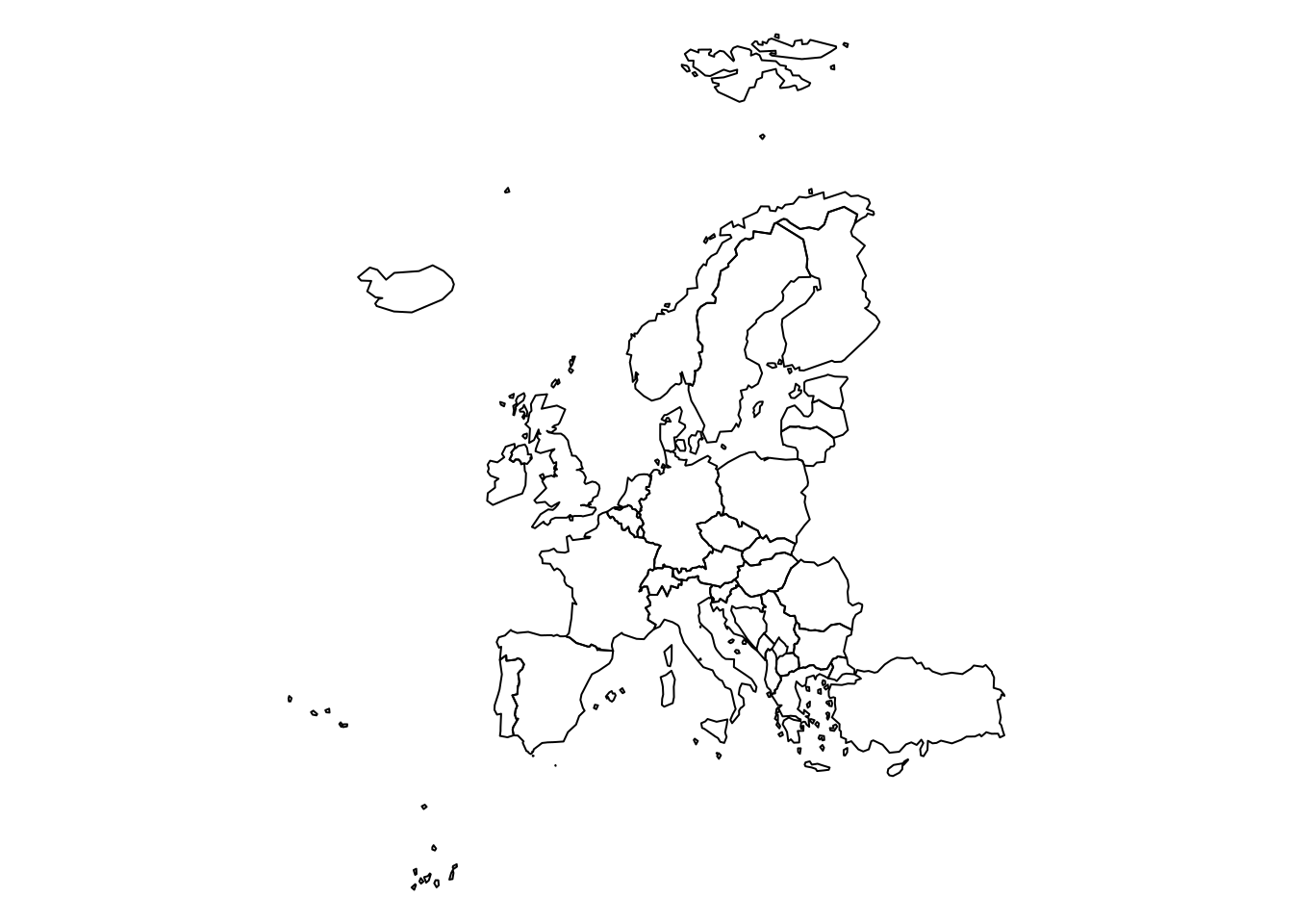
Create an "sts" object (DIY)
Using the above ingredients (ecdc, pop,
map) and knowing that the monthly ecdc time
series starts at
[1] 1999 1you can now create an "sts" object via the constructor
function sts().
Lade nötiges Paket: xtableThis is surveillance 1.23.1; see 'package?surveillance' or
https://surveillance.R-Forge.R-project.org/ for an overview.## See help("sts") and learn about the function arguments:
str(sts)
## Complete the following expression:
## IMD <- sts(....)Solution
It should give the following printed output:
-- An object of class sts --
freq:        12
start:       1999 1
dim(observed):   240 17

Head of observed:
     AT CZ DE DK EE EL  ES FI FR IE IS IT NL NO PL SI  UK
[1,] 11  5 37 19  0 18 172  6 43 53  2 36 81  4 11  1 495

map: 37 Polygons, without data
Try some methods
Try some of the methods for "sts" objects with the
IMD dataset, see Section
“Methods” in help(sts).
Extraction
Try:
dim(),colnames()epoch(),epochInYear(),year()observed(),population()
Solution
[1] 240 17 [1] "AT" "CZ" "DE" "DK" "EE" "EL" "ES" "FI" "FR" "IE" "IS" "IT" "NL" "NO" "PL" "SI" "UK" [1] "1999-01-01" "1999-02-01" "1999-03-01" "1999-04-01" "1999-05-01" "1999-06-01" "1999-07-01"
[8] "1999-08-01" "1999-09-01" "1999-10-01" "1999-11-01" "1999-12-01" "2000-01-01" "2000-02-01"
[15] "2000-03-01" "2000-04-01" "2000-05-01" "2000-06-01" "2000-07-01" "2000-08-01" "2000-09-01"
[22] "2000-10-01" "2000-11-01" "2000-12-01" "2001-01-01" "2001-02-01" "2001-03-01" "2001-04-01"
[29] "2001-05-01" "2001-06-01" "2001-07-01" "2001-08-01" "2001-09-01" "2001-10-01" "2001-11-01"
[36] "2001-12-01" "2002-01-01" "2002-02-01" "2002-03-01" "2002-04-01" "2002-05-01" "2002-06-01"
[43] "2002-07-01" "2002-08-01" "2002-09-01" "2002-10-01" "2002-11-01" "2002-12-01" "2003-01-01"
[50] "2003-02-01" "2003-03-01" "2003-04-01" "2003-05-01" "2003-06-01" "2003-07-01" "2003-08-01"
[57] "2003-09-01" "2003-10-01" "2003-11-01" "2003-12-01" "2004-01-01" "2004-02-01" "2004-03-01"
[64] "2004-04-01" "2004-05-01" "2004-06-01" "2004-07-01" "2004-08-01" "2004-09-01" "2004-10-01"
[71] "2004-11-01" "2004-12-01" "2005-01-01" "2005-02-01" "2005-03-01" "2005-04-01" "2005-05-01"
[78] "2005-06-01" "2005-07-01" "2005-08-01" "2005-09-01" "2005-10-01" "2005-11-01" "2005-12-01"
[85] "2006-01-01" "2006-02-01" "2006-03-01" "2006-04-01" "2006-05-01" "2006-06-01" "2006-07-01"
[92] "2006-08-01" "2006-09-01" "2006-10-01" "2006-11-01" "2006-12-01" "2007-01-01" "2007-02-01"
[99] "2007-03-01" "2007-04-01" "2007-05-01" "2007-06-01" "2007-07-01" "2007-08-01" "2007-09-01"
[106] "2007-10-01" "2007-11-01" "2007-12-01" "2008-01-01" "2008-02-01" "2008-03-01" "2008-04-01"
[113] "2008-05-01" "2008-06-01" "2008-07-01" "2008-08-01" "2008-09-01" "2008-10-01" "2008-11-01"
[120] "2008-12-01" "2009-01-01" "2009-02-01" "2009-03-01" "2009-04-01" "2009-05-01" "2009-06-01"
[127] "2009-07-01" "2009-08-01" "2009-09-01" "2009-10-01" "2009-11-01" "2009-12-01" "2010-01-01"
[134] "2010-02-01" "2010-03-01" "2010-04-01" "2010-05-01" "2010-06-01" "2010-07-01" "2010-08-01"
[141] "2010-09-01" "2010-10-01" "2010-11-01" "2010-12-01" "2011-01-01" "2011-02-01" "2011-03-01"
[148] "2011-04-01" "2011-05-01" "2011-06-01" "2011-07-01" "2011-08-01" "2011-09-01" "2011-10-01"
[155] "2011-11-01" "2011-12-01" "2012-01-01" "2012-02-01" "2012-03-01" "2012-04-01" "2012-05-01"
[162] "2012-06-01" "2012-07-01" "2012-08-01" "2012-09-01" "2012-10-01" "2012-11-01" "2012-12-01"
[169] "2013-01-01" "2013-02-01" "2013-03-01" "2013-04-01" "2013-05-01" "2013-06-01" "2013-07-01"
[176] "2013-08-01" "2013-09-01" "2013-10-01" "2013-11-01" "2013-12-01" "2014-01-01" "2014-02-01"
[183] "2014-03-01" "2014-04-01" "2014-05-01" "2014-06-01" "2014-07-01" "2014-08-01" "2014-09-01"
[190] "2014-10-01" "2014-11-01" "2014-12-01" "2015-01-01" "2015-02-01" "2015-03-01" "2015-04-01"
[197] "2015-05-01" "2015-06-01" "2015-07-01" "2015-08-01" "2015-09-01" "2015-10-01" "2015-11-01"
[204] "2015-12-01" "2016-01-01" "2016-02-01" "2016-03-01" "2016-04-01" "2016-05-01" "2016-06-01"
[211] "2016-07-01" "2016-08-01" "2016-09-01" "2016-10-01" "2016-11-01" "2016-12-01" "2017-01-01"
[218] "2017-02-01" "2017-03-01" "2017-04-01" "2017-05-01" "2017-06-01" "2017-07-01" "2017-08-01"
[225] "2017-09-01" "2017-10-01" "2017-11-01" "2017-12-01" "2018-01-01" "2018-02-01" "2018-03-01"
[232] "2018-04-01" "2018-05-01" "2018-06-01" "2018-07-01" "2018-08-01" "2018-09-01" "2018-10-01"
[239] "2018-11-01" "2018-12-01" [1] 1999 1999 1999 1999 1999 1999 1999 1999 1999 1999 1999 1999 2000 2000 2000 2000 2000 2000
[19] 2000 2000 2000 2000 2000 2000 2001 2001 2001 2001 2001 2001 2001 2001 2001 2001 2001 2001
[37] 2002 2002 2002 2002 2002 2002 2002 2002 2002 2002 2002 2002 2003 2003 2003 2003 2003 2003
[55] 2003 2003 2003 2003 2003 2003 2004 2004 2004 2004 2004 2004 2004 2004 2004 2004 2004 2004
[73] 2005 2005 2005 2005 2005 2005 2005 2005 2005 2005 2005 2005 2006 2006 2006 2006 2006 2006
[91] 2006 2006 2006 2006 2006 2006 2007 2007 2007 2007 2007 2007 2007 2007 2007 2007 2007 2007
[109] 2008 2008 2008 2008 2008 2008 2008 2008 2008 2008 2008 2008 2009 2009 2009 2009 2009 2009
[127] 2009 2009 2009 2009 2009 2009 2010 2010 2010 2010 2010 2010 2010 2010 2010 2010 2010 2010
[145] 2011 2011 2011 2011 2011 2011 2011 2011 2011 2011 2011 2011 2012 2012 2012 2012 2012 2012
[163] 2012 2012 2012 2012 2012 2012 2013 2013 2013 2013 2013 2013 2013 2013 2013 2013 2013 2013
[181] 2014 2014 2014 2014 2014 2014 2014 2014 2014 2014 2014 2014 2015 2015 2015 2015 2015 2015
[199] 2015 2015 2015 2015 2015 2015 2016 2016 2016 2016 2016 2016 2016 2016 2016 2016 2016 2016
[217] 2017 2017 2017 2017 2017 2017 2017 2017 2017 2017 2017 2017 2018 2018 2018 2018 2018 2018
[235] 2018 2018 2018 2018 2018 2018 [1] 1 2 3 4 5 6 7 8 9 10 11 12 1 2 3 4 5 6 7 8 9 10 11 12 1 2 3 4 5 6 7
[32] 8 9 10 11 12 1 2 3 4 5 6 7 8 9 10 11 12 1 2 3 4 5 6 7 8 9 10 11 12 1 2
[63] 3 4 5 6 7 8 9 10 11 12 1 2 3 4 5 6 7 8 9 10 11 12 1 2 3 4 5 6 7 8 9
[94] 10 11 12 1 2 3 4 5 6 7 8 9 10 11 12 1 2 3 4 5 6 7 8 9 10 11 12 1 2 3 4
[125] 5 6 7 8 9 10 11 12 1 2 3 4 5 6 7 8 9 10 11 12 1 2 3 4 5 6 7 8 9 10 11
[156] 12 1 2 3 4 5 6 7 8 9 10 11 12 1 2 3 4 5 6 7 8 9 10 11 12 1 2 3 4 5 6
[187] 7 8 9 10 11 12 1 2 3 4 5 6 7 8 9 10 11 12 1 2 3 4 5 6 7 8 9 10 11 12 1
[218] 2 3 4 5 6 7 8 9 10 11 12 1 2 3 4 5 6 7 8 9 10 11 12 AT CZ DE DK EE EL ES FI FR IE IS IT NL NO PL SI UK
[1,] 11 5 37 19 0 18 172 6 43 53 2 36 81 4 11 1 495
[2,] 14 8 48 17 0 16 123 9 65 43 2 31 68 11 9 0 267
[3,] 12 11 54 28 0 42 90 5 35 53 1 29 82 10 8 0 224
[4,] 6 9 36 22 1 21 70 3 30 40 2 23 33 4 4 1 203
[5,] 3 14 36 11 0 16 78 7 18 34 2 18 41 6 6 1 140
[6,] 4 10 30 12 0 11 50 8 19 24 2 21 38 4 1 0 199 AT CZ DE DK EE EL ES FI FR IE IS
[1,] 8822267 10610055 82792351 5781190 1319133 10741165 46658447 5513130 67026224 4830392 348450
[2,] 8822267 10610055 82792351 5781190 1319133 10741165 46658447 5513130 67026224 4830392 348450
[3,] 8822267 10610055 82792351 5781190 1319133 10741165 46658447 5513130 67026224 4830392 348450
[4,] 8822267 10610055 82792351 5781190 1319133 10741165 46658447 5513130 67026224 4830392 348450
[5,] 8822267 10610055 82792351 5781190 1319133 10741165 46658447 5513130 67026224 4830392 348450
[6,] 8822267 10610055 82792351 5781190 1319133 10741165 46658447 5513130 67026224 4830392 348450
IT NL NO PL SI UK
[1,] 60483973 17181084 5295619 37976687 2066880 66273576
[2,] 60483973 17181084 5295619 37976687 2066880 66273576
[3,] 60483973 17181084 5295619 37976687 2066880 66273576
[4,] 60483973 17181084 5295619 37976687 2066880 66273576
[5,] 60483973 17181084 5295619 37976687 2066880 66273576
[6,] 60483973 17181084 5295619 37976687 2066880 66273576Class "sts" [package "surveillance"]
Slots:
Name: epoch freq start observed state
Class: numeric numeric numeric matrix matrix
Name: alarm upperbound neighbourhood populationFrac map
Class: matrix matrix matrix matrix SpatialPolygons
Name: control epochAsDate multinomialTS
Class: list logical logical
Known Subclasses: "stsBP", "stsNC"Subsetting
Try some ways of subsetting the multivariate time series using conventional indexing for matrix-like objects:
[i,j]
Solution
-- An object of class sts --
freq:        12
start:       1999 1
dim(observed):   3 1

Head of observed:
      UK
[1,] 495

map: 37 Polygons, without data-- An object of class sts --
freq: 12
start: 2018 1
dim(observed): 12 17
Head of observed:
AT CZ DE DK EE EL ES FI FR IE IS IT NL NO PL SI UK
[1,] 4 3 34 3 0 4 72 0 75 21 0 38 22 2 16 3 158
map: 37 Polygons, without data-- An object of class sts --
freq: 12
start: 2012 1
dim(observed): 84 17
Head of observed:
AT CZ DE DK EE EL ES FI FR IE IS IT NL NO PL SI UK
[1,] 5 9 44 8 0 4 61 3 58 13 1 17 13 4 29 1 119
map: 37 Polygons, without dataTo keep things simple, you may wish to restrict some of the following
exercises to an (arbitrary) subset of 6 countries;
let’s use those whose country code starts with one of the letters D, F,
or N. Create this subset and name the object IMD6.
Conversion
Try:
aggregate(), see?aggregate.stsas.data.frame(), possibly with argumenttidy = TRUE(ortidy.sts())as.ts()
Solution
## collapse the multivariate time series in either dimension
## help(aggregate.sts)
aggregate(IMD6, by = "time")  # summing over time
-- An object of class sts --
freq: 240
start: 1999 1
dim(observed): 1 6
Head of observed:
DE DK FI FR NL NO
[1,] 9184 1575 679 11250 5174 785
map: 37 Polygons, without data-- An object of class sts --
freq: 12
start: 1999 1
dim(observed): 240 1
Head of observed:
overall
[1,] 190## convert to a data frame (omitting non-temporal slots)
as.data.frame(IMD6) |> head(3) # wide format observed.DE observed.DK observed.FI observed.FR observed.NL observed.NO epoch state.DE state.DK
1 37 19 6 43 81 4 1 FALSE FALSE
2 48 17 9 65 68 11 2 FALSE FALSE
3 54 28 5 35 82 10 3 FALSE FALSE
state.FI state.FR state.NL state.NO alarm.DE alarm.DK alarm.FI alarm.FR alarm.NL alarm.NO
1 FALSE FALSE FALSE FALSE NA NA NA NA NA NA
2 FALSE FALSE FALSE FALSE NA NA NA NA NA NA
3 FALSE FALSE FALSE FALSE NA NA NA NA NA NA
upperbound.DE upperbound.DK upperbound.FI upperbound.FR upperbound.NL upperbound.NO
1 NA NA NA NA NA NA
2 NA NA NA NA NA NA
3 NA NA NA NA NA NA
population.DE population.DK population.FI population.FR population.NL population.NO freq
1 82792351 5781190 5513130 67026224 17181084 5295619 12
2 82792351 5781190 5513130 67026224 17181084 5295619 12
3 82792351 5781190 5513130 67026224 17181084 5295619 12
epochInPeriod
1 0.08333333
2 0.16666667
3 0.25000000 epoch unit year freq epochInYear epochInPeriod date observed state alarm upperbound
1 1 DE 1999 12 1 0.08333333 1999-01-01 37 FALSE NA NA
2 2 DE 1999 12 2 0.16666667 1999-02-01 48 FALSE NA NA
3 3 DE 1999 12 3 0.25000000 1999-03-01 54 FALSE NA NA
population
1 82792351
2 82792351
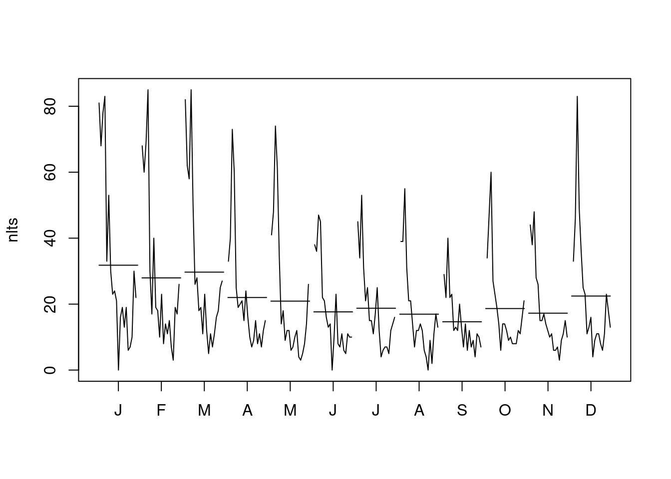
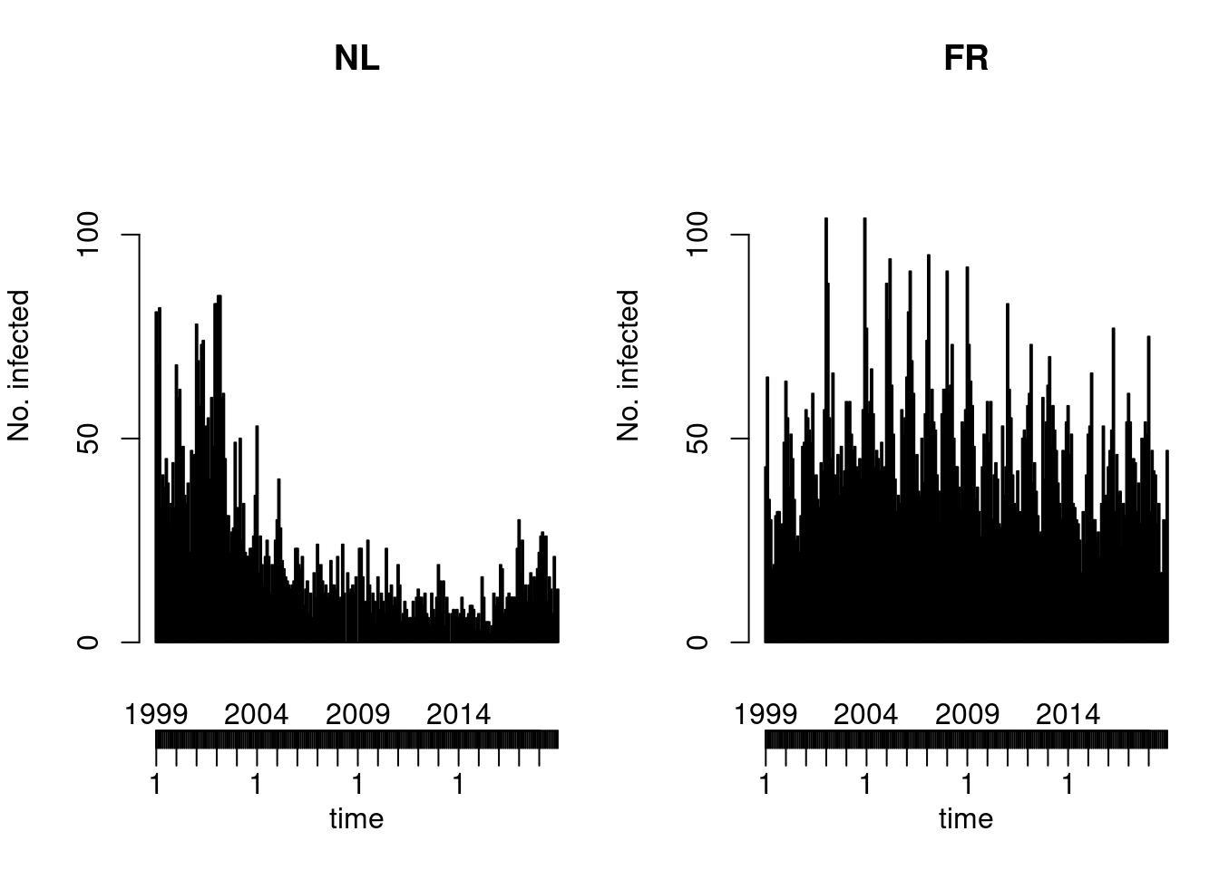
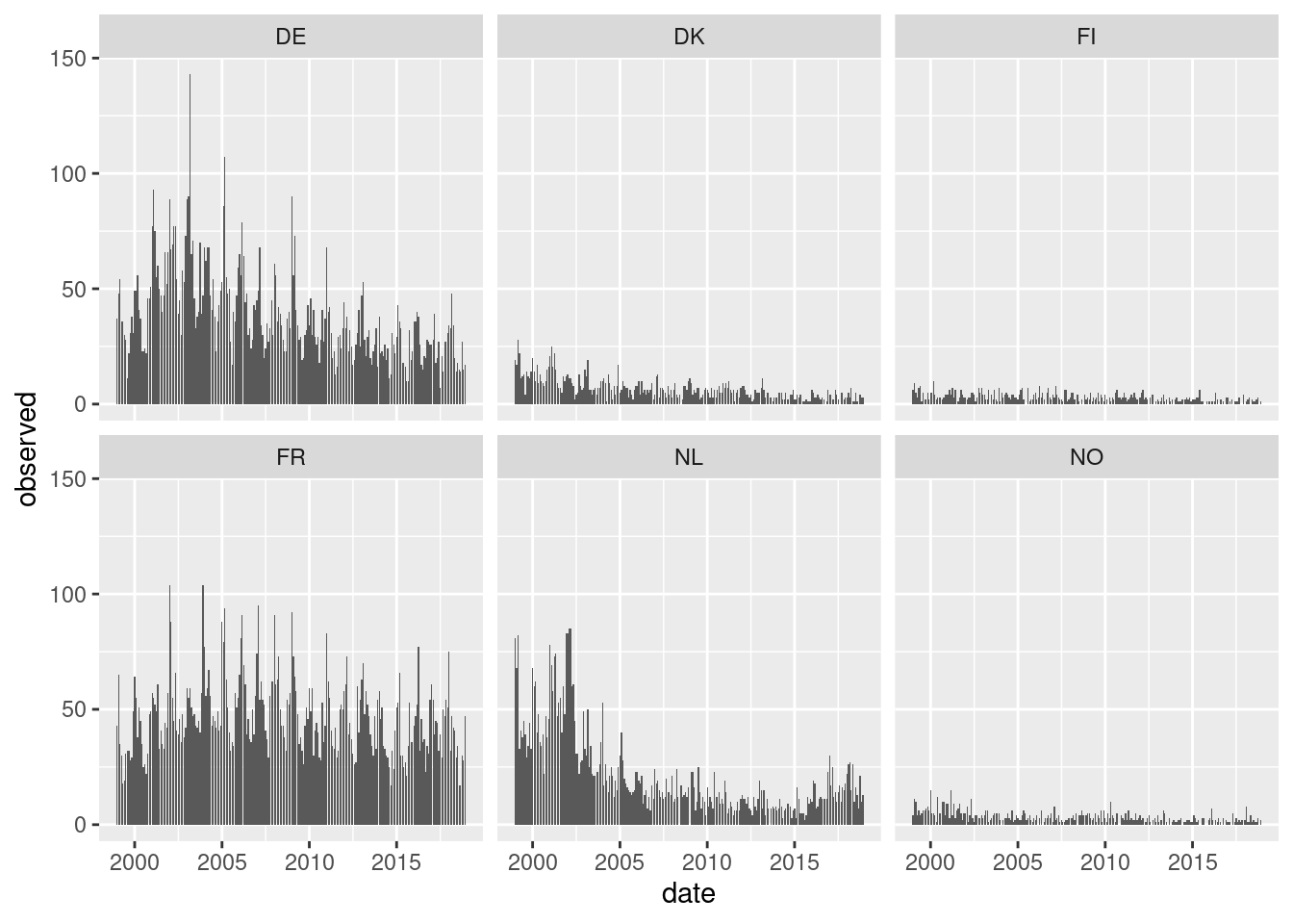
3 82792351IMD6DF <- tidy.sts(IMD6) # the same
## the long data format is convenient for, e.g., custom 'lattice' plots
lattice::xyplot(observed ~ date | unit, data = IMD6DF, type = "h", as.table = TRUE)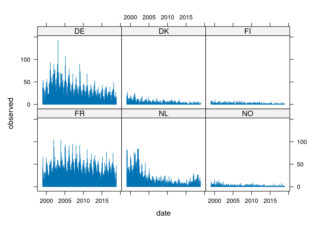
         DE DK FI FR NL NO
Jan 1999 37 19  6 43 81  4
Feb 1999 48 17  9 65 68 11
Mar 1999 54 28  5 35 82 10
Apr 1999 36 22  3 30 33  4
May 1999 36 11  7 18 41  6
Jun 1999 30 12  8 19 38  4
Jul 1999 28 13  1 31 45  5
Aug 1999 11  4  5 32 39  6
Sep 1999 22 14  2 32 29  6
Oct 1999 31 12  2 28 34  7
Nov 1999 38 11  5 29 44  8
Dec 1999 31 14  2 49 33  6
Jan 2000 49 20  5 64 68 15
Feb 2000 49 14  5 55 60  5
Mar 2000 56 10 10 38 62  5
Apr 2000 41 17  4 51 40  4
May 2000 37  9  2 45 48  1
Jun 2000 23 13  3 35 36 12
Jul 2000 23 10  3 25 34  5
Aug 2000 24  9  3 26 39  5
Sep 2000 22  8  2 22 22 10
Oct 2000 46 10  3 31 47 10
Nov 2000 46 15  4 48 38  4
Dec 2000 51 16 4 49 46 9 Jan Feb Mar Apr May Jun Jul Aug Sep Oct Nov Dec
1999 81 68 82 33 41 38 45 39 29 34 44 33
2000 68 60 62 40 48 36 34 39 22 47 38 46
2001 78 69 58 73 74 47 53 55 40 60 48 83
2002 83 85 85 60 61 45 31 31 22 27 28 49
2003 33 30 50 25 34 22 21 21 23 23 26 36
2004 53 17 26 19 14 21 25 21 12 19 15 25
2005 30 40 28 20 18 16 15 14 13 14 15 23
2006 23 19 18 21 9 13 15 7 12 6 17 11
2007 24 18 19 15 12 14 11 12 20 14 14 13
2008 21 10 11 24 12 0 17 12 13 14 12 16
2009 0 23 23 16 6 10 25 14 7 12 10 4
2010 16 8 12 10 7 23 12 12 14 9 11 9
2011 19 14 5 7 10 8 4 6 6 10 6 11
2012 13 11 11 9 12 7 6 4 12 8 6 11
2013 19 15 7 15 4 11 7 0 7 8 7 8
2014 6 7 11 8 3 6 7 9 9 8 3 6
2015 7 3 16 11 5 5 5 2 4 12 9 11
2016 10 19 18 7 8 11 12 11 11 11 11 23
2017 30 17 25 12 14 10 14 17 10 16 15 18
2018 22 26 27 15 26 10 16 13 7 21 10 13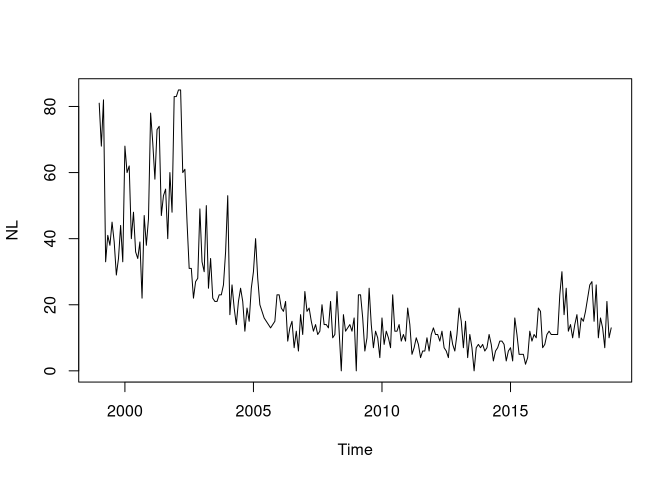
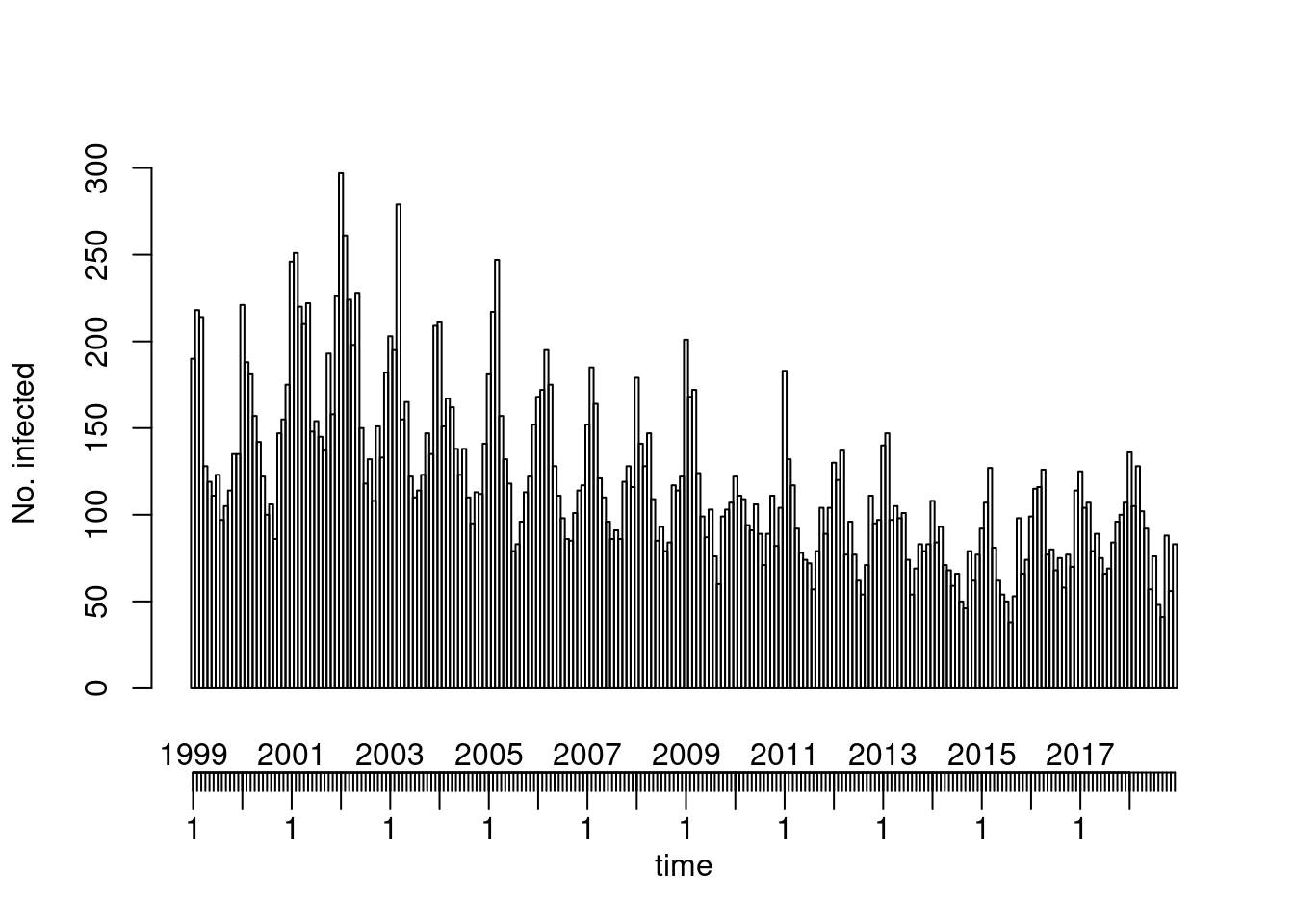
## if you have package 'xts', this also works:
xts::as.xts(IMD6) |> # then using the plot-method from 'xts'
    plot(multi.panel = TRUE, yaxis.same = FALSE)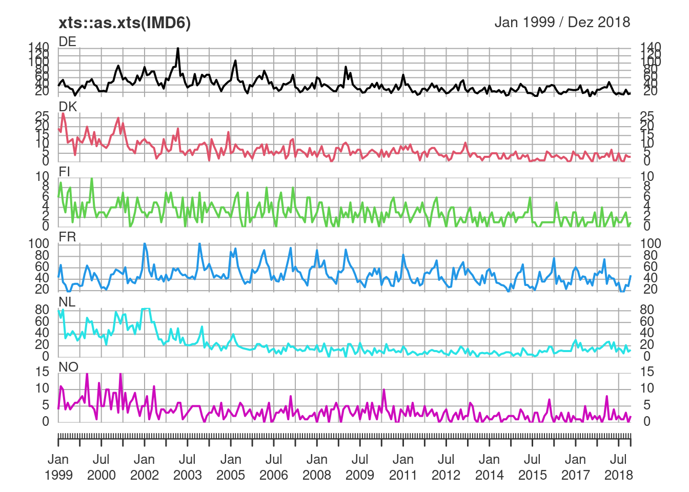
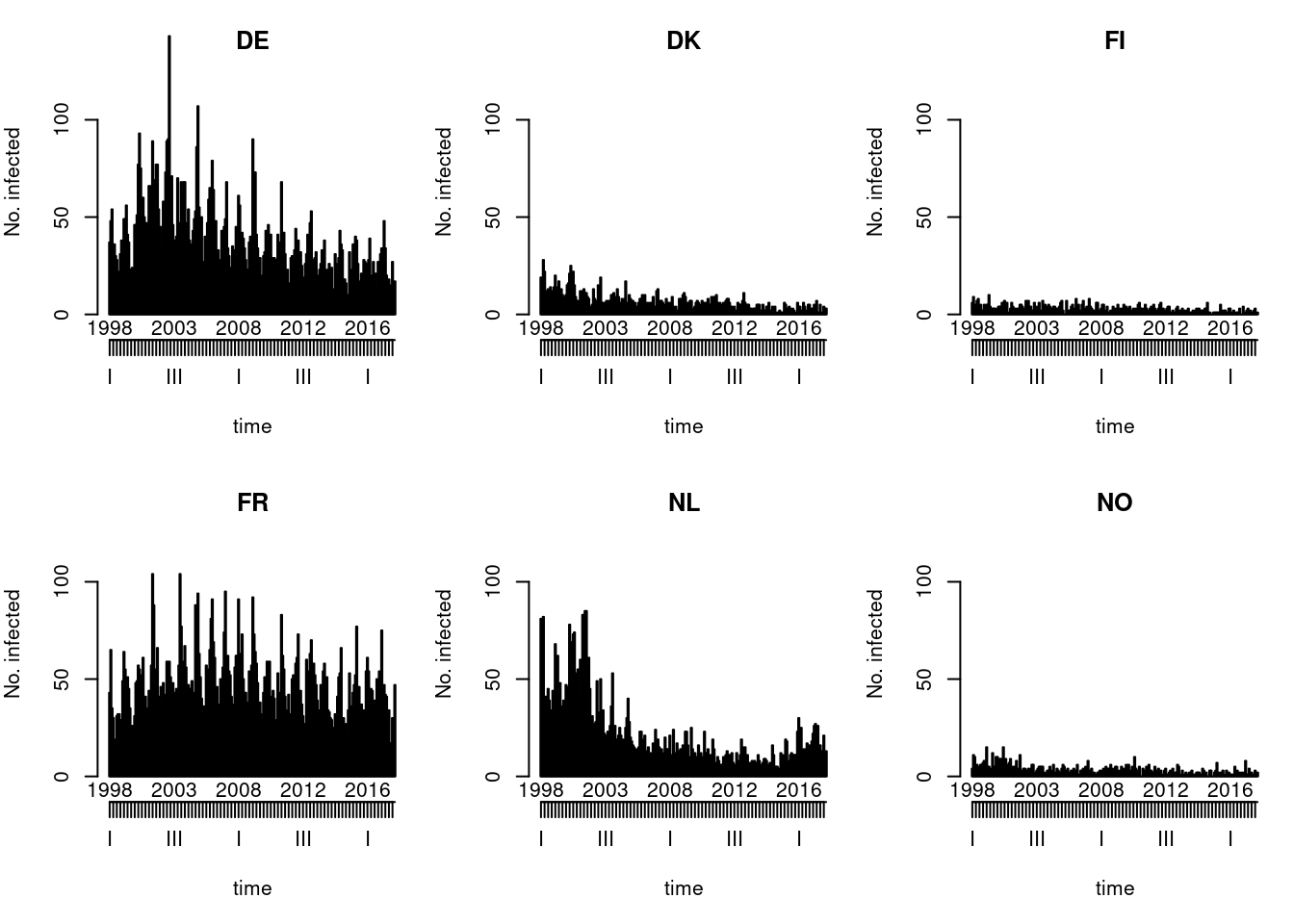
Visualization
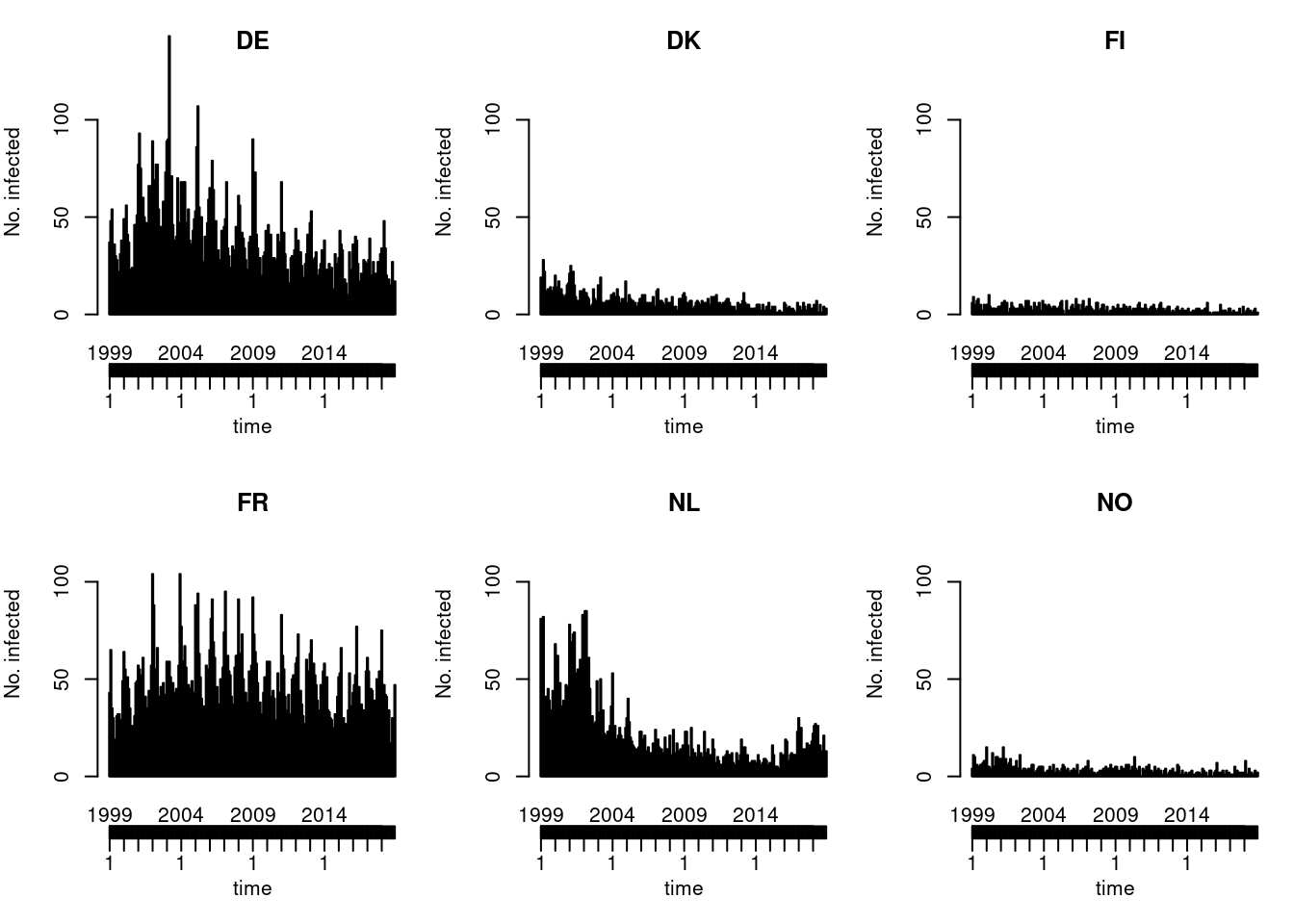
Try plot(IMD6), but see help(plot.sts)
for an overview of the different types of plots available.
The various plot types should provide enough functionality for common
visualization needs. More sophisticated plots can always be crafted as
needed, based on the provided methods or following
as.data.frame(<sts>).
Default type (observed ~ time | unit)
Solution
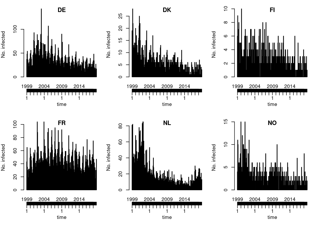
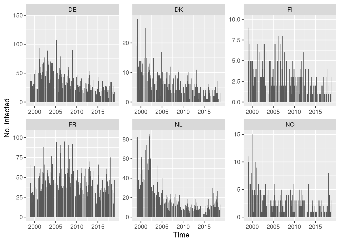
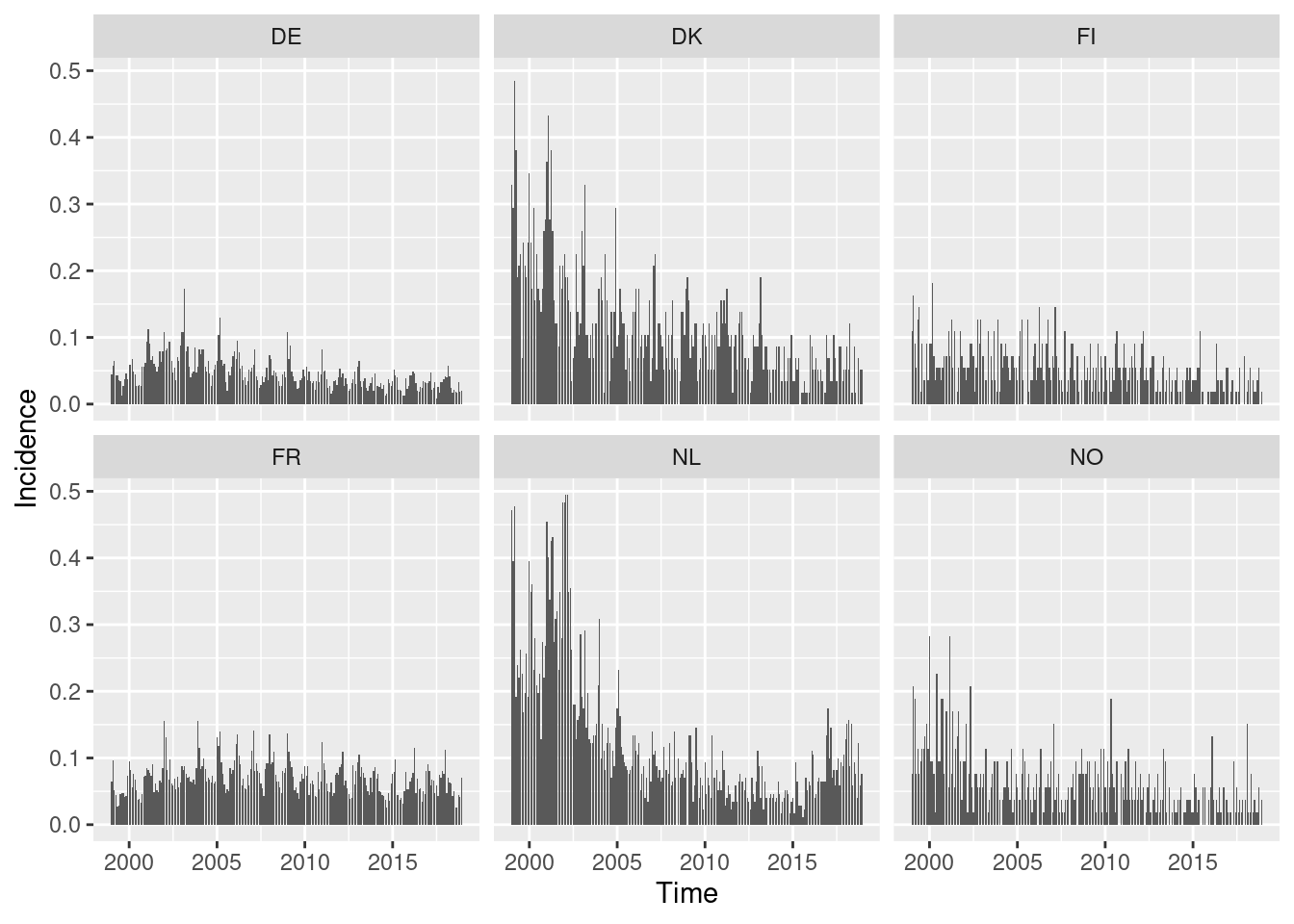
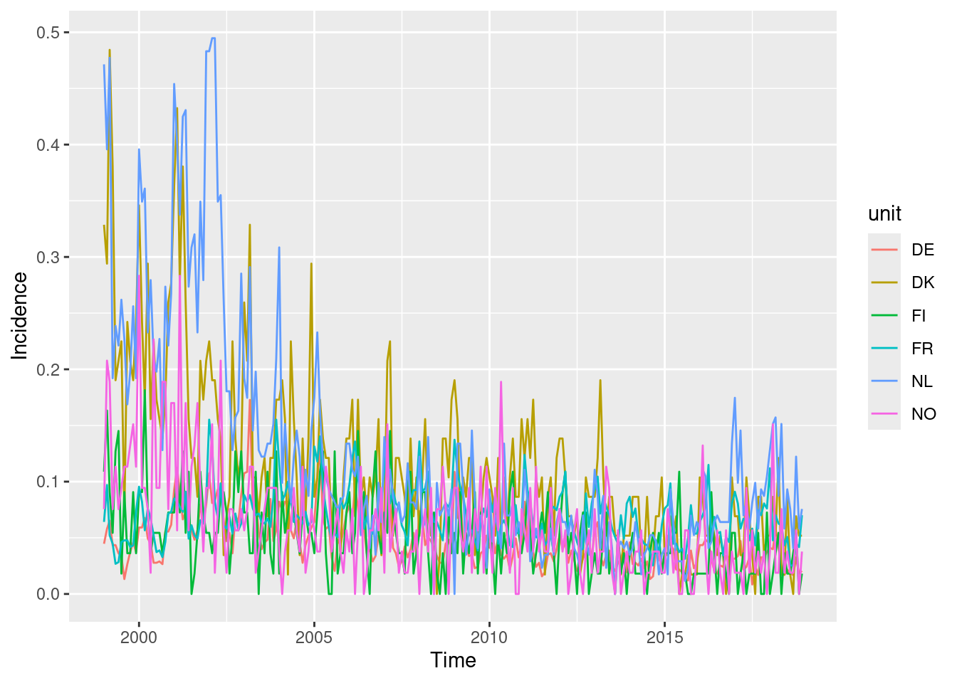
You could also try the ggplot2 version of this plot
using autoplot.sts().
This allows incidences to be plotted rather than counts.

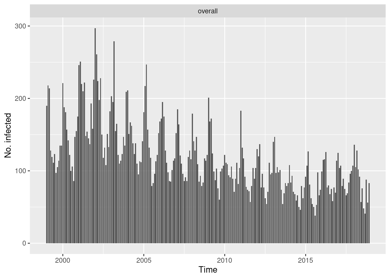
Overall (observed ~ time)
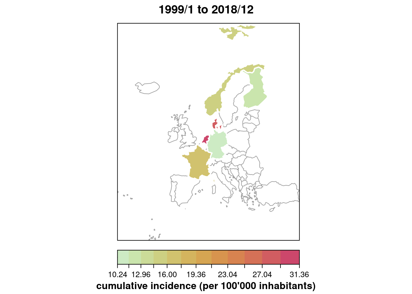
Map (observed ~ unit)
Produce a map with the country-specific cumulative number of cases
(or incidence) over time. See help("stsplot_space") for
options.
Solution
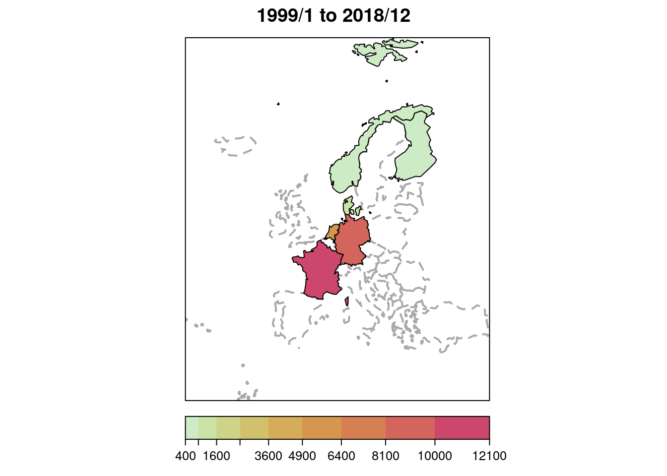
## only for the year 2018
plot(IMD6, type = observed ~ unit,
     tps = which(year(IMD6) == 2018),
     total.args = list()) # annotate with total number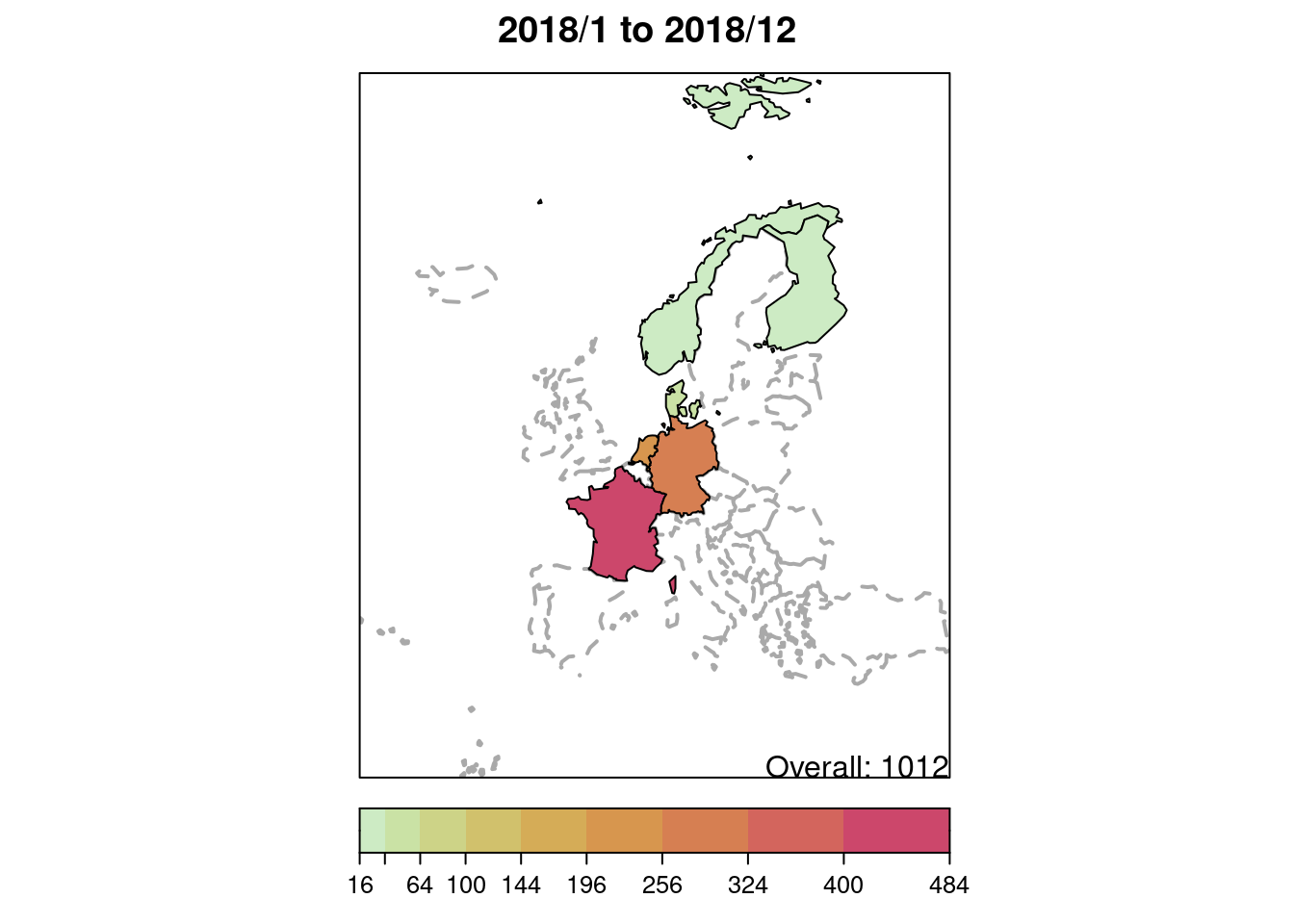
## cumulative incidence (per 100'000 inhabitants),
## using some of the graphical options
plot(IMD6, type = observed ~ unit, population = 100000,
     gpar.missing = list(lty = 1, col = 8),
     col = "white", lwd = 2, # thick white borders
     sub = "cumulative incidence (per 100'000 inhabitants)")