Tutorial 1: Univariate
hhh4()
Using weekly counts of norovirus gastroenteritis from Berlin
Template: univariate.R
Abstract
This tutorial introduces endemic-epidemic models using a single time
series of counts. Univariate analyses are not the main target of
hhh4() and many other tools exist for this simple case, but
it can serve as an accessible first encounter of the modelling concept.
We use data on weekly counts of norovirus infections in Berlin, Germany,
readily provided as an "sts" object for use with the
surveillance package. If you wish to learn more about
this specific data class and available methods, see the "sts" tutorial. The same dataset is
also used in the multivariate tutorial,
but then disaggregated by district.
Some initial code is provided in the R script template
univariate.R that is part of the tutorials.zip
archive, as are the necessary data files.
Data
We use data from routine surveillance in Germany carried out by Robert Koch Institute. We have
already prepared these as "sts" (surveillance time
series) data, which you can directly load from the provided RData file.
Lade nötiges Paket: spLade nötiges Paket: xtableThis is surveillance 1.23.1; see 'package?surveillance' or
https://surveillance.R-Forge.R-project.org/ for an overview.Loading objects:
noroBE
rotaBEWe focus on noroBE, which contains weekly counts of
confirmed cases of norovirus
gastroenteritis in Berlin, 2011–2017, stratified by district. These
data have already been used as an example in at least two publications
on hhh4 extensions (for serial interval
distributions and social contact
data, respectively).
The rotaBE dataset contains the same for rotavirus
gastroenteritis, which you can explore if you want to play around a
bit more.
In this tutorial, we only look at the overall time series aggregated over all districts:
-- An object of class sts --
freq:        52
start:       2011 1
dim(observed):   364 1

Head of observed:
     overall
[1,]     157
Task
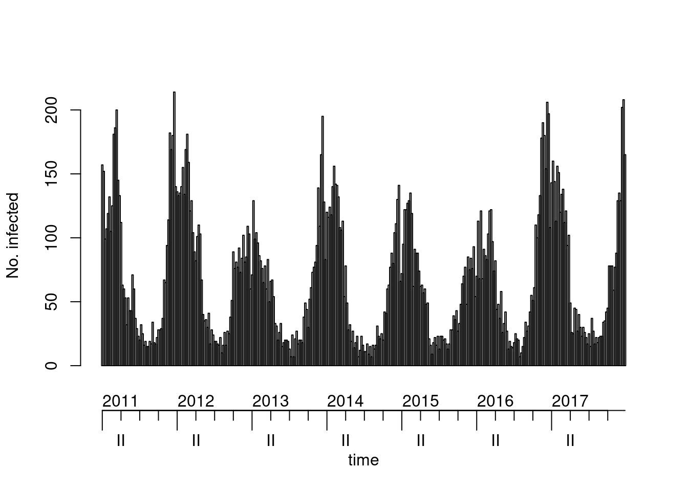
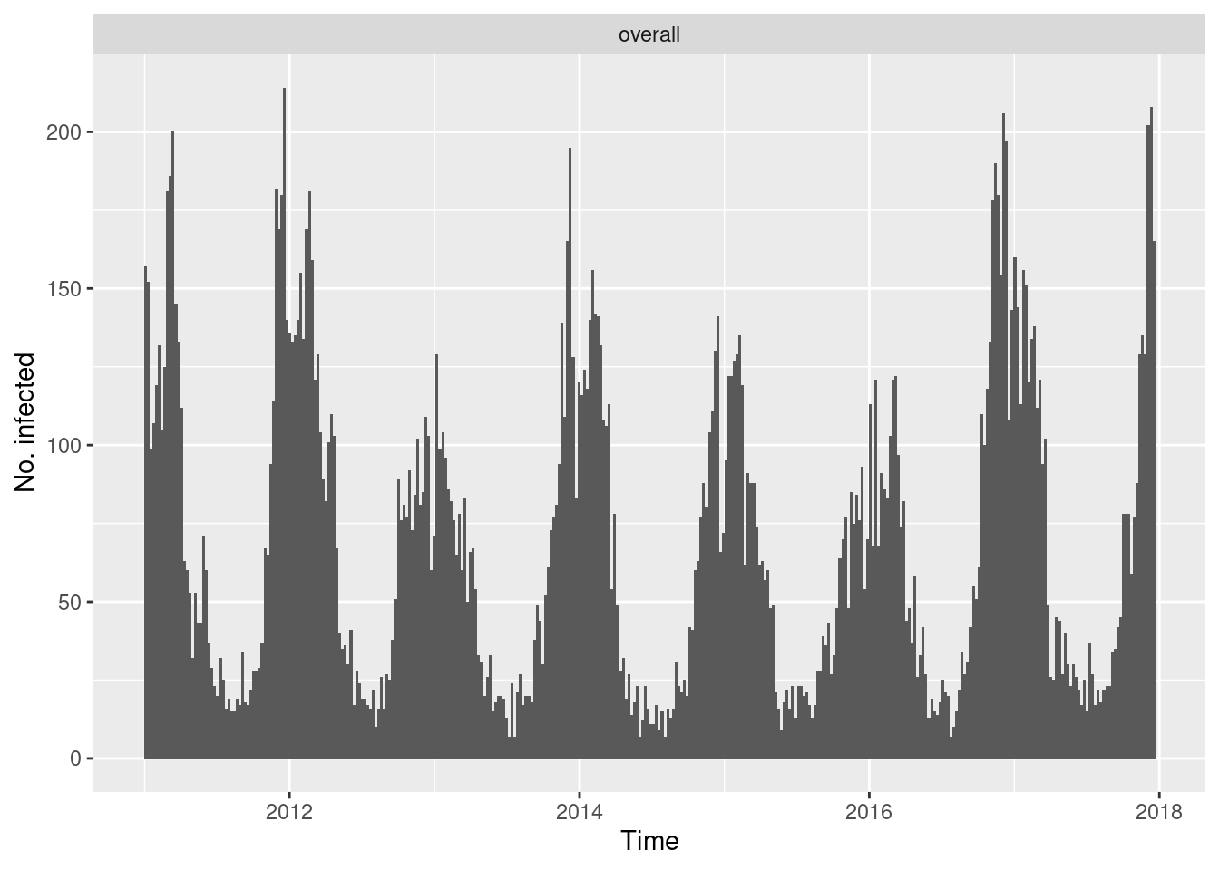
Look at a plot() of the data. You can also try a
ggplot2 version via ggplot2::autoplot(),
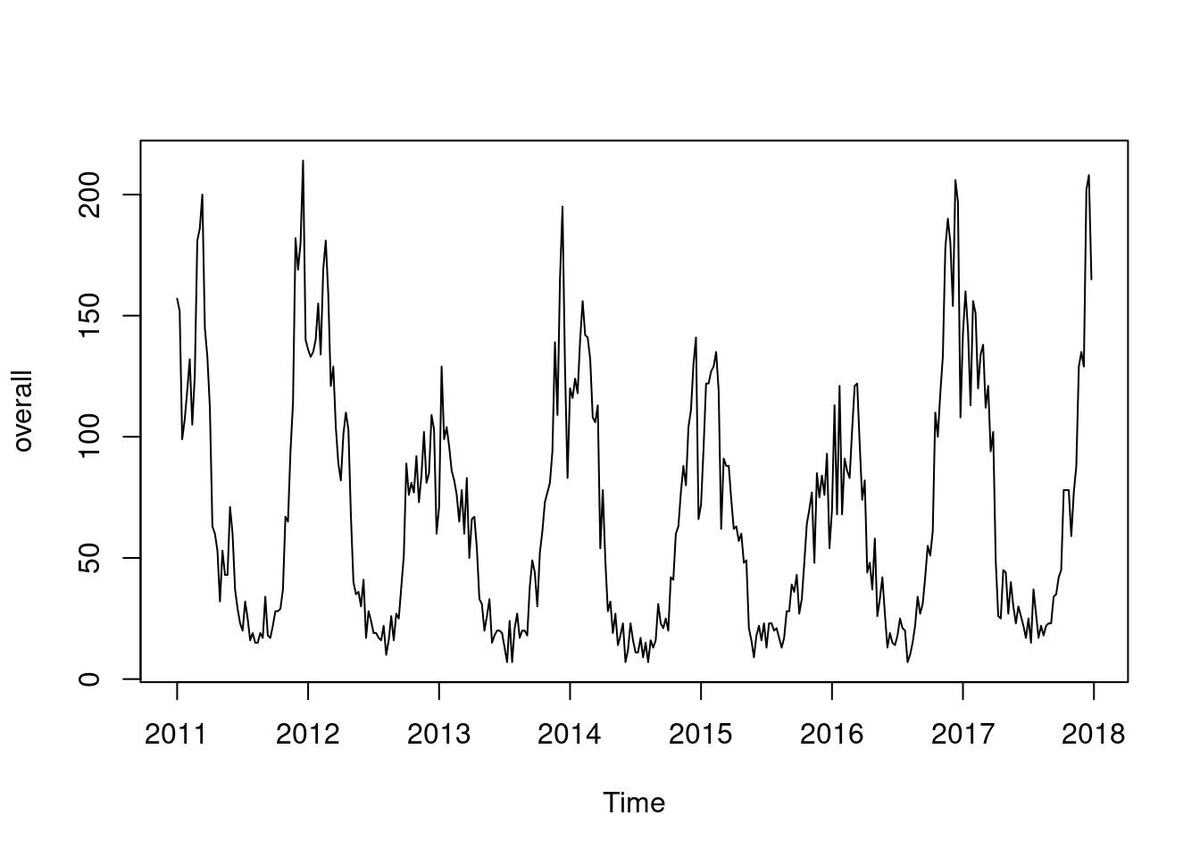
or plot an as.ts() or xts::as.xts() (if you
have that) version of the data.
Alternatively, convert the "sts" object to a “tidy” data
frame via tidy.sts() and use your favourite plotting
tool.
Solution
## alternative visualizations (and there are probably more)
plot(noro, col = 8, epochsAsDate = TRUE)  # alternative colour & time axis setup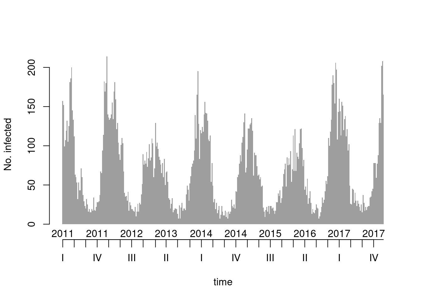
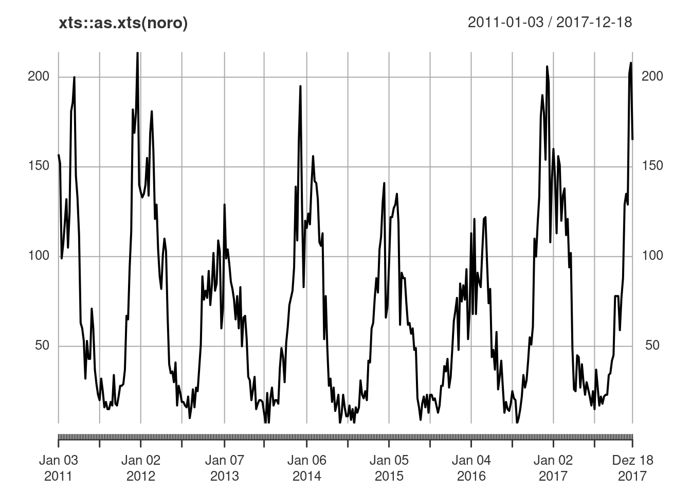
## there is a clear yearly seasonality, see also
## the basic "ts" monthplot()
as.ts(noro) |> monthplot(lwd.base = 3)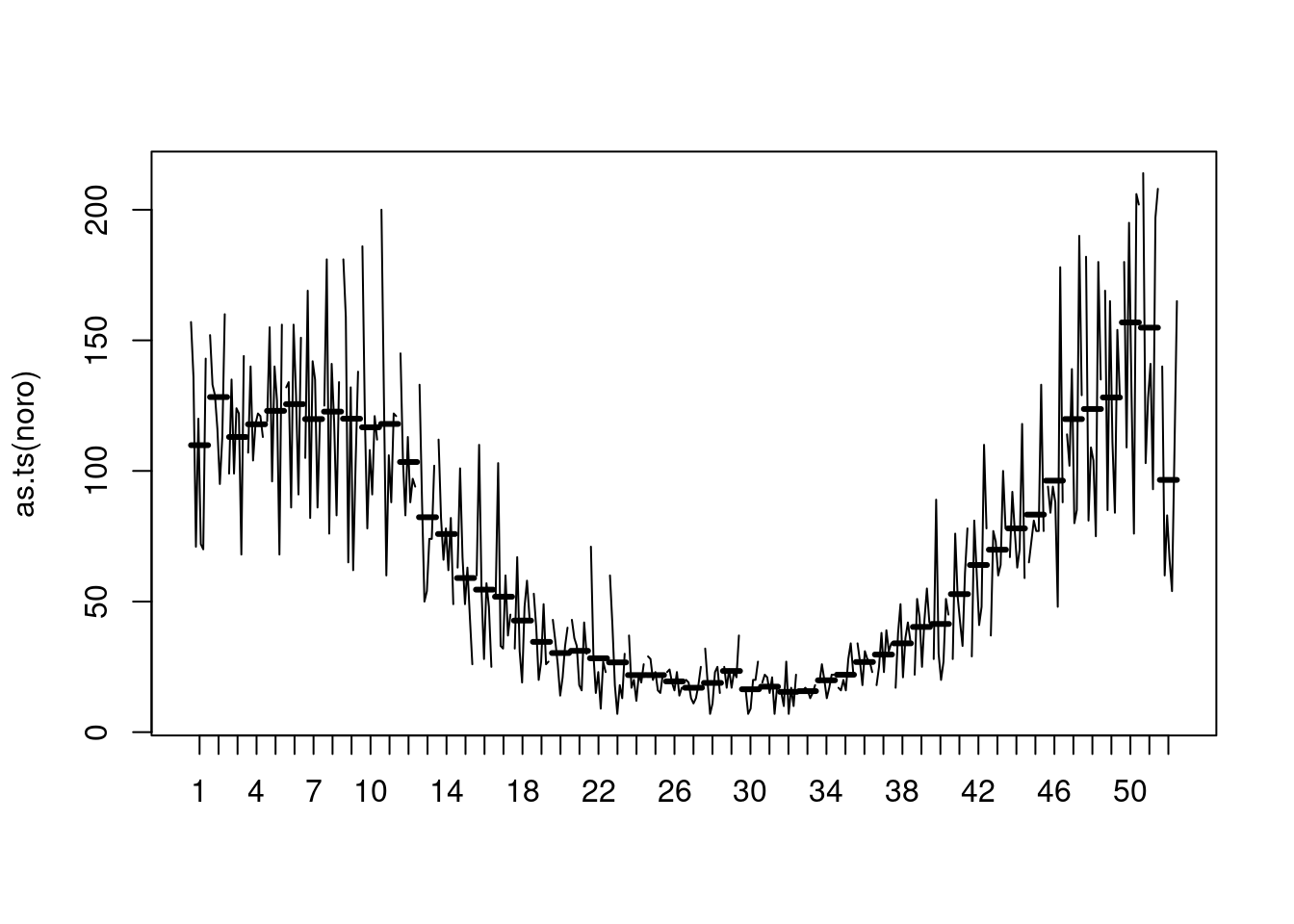
## => (unfortunate) peak around Christmas, minimum around calendar week 32

## or use, e.g., lattice::xyplot() with the "tidy" dataset
lattice::xyplot(observed ~ epochInYear, data = tidy.sts(noro),
                groups = year, type = "l", xlab = "calendar week")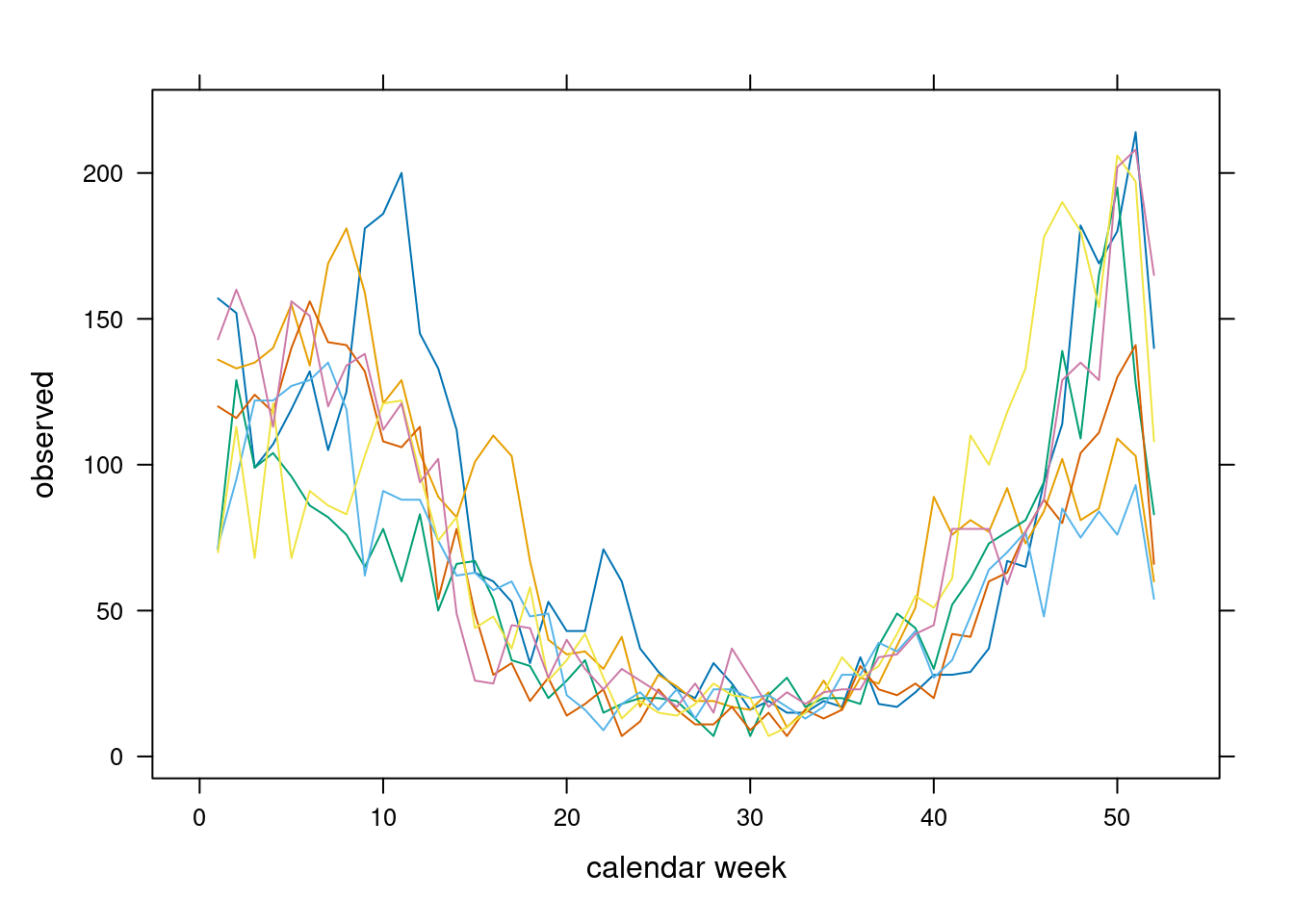
Fitting hhh4() models
We don’t have any exogenous covariates in this example, but we can at least capture seasonality by including transformations of time (pairs of sine-cosine terms) as covariates in the model.
In statistical terms, we will fit simple models of the form
\[ Y_t | Y_{t-1} \sim \operatorname{NegBin}(\nu_t + \lambda_t y_{t-1}, \phi) \]
where the log-linear predictors \(\nu_t\) (endemic component)
and \(\lambda_t\) (ar
component) could use regression formulae of the form
\[ \alpha + \sum_{s=1}^S \left\{ \gamma_s \sin(s \omega t) + \delta_s \cos(s \omega t) \right\} \]
with S harmonics of “fundamental frequency” \(\omega=2\pi/52\).
Such a formula for use in hhh4() model
components can be created very easily, here adding just one harmonic to
an intercept-only formula:
~1 + sin(2 * pi * t/52) + cos(2 * pi * t/52)The basic syntax for fitting an endemic-epidemic time-series model is
where the first argument gives the data as an "sts"
object (here: noro) and the second argument specifies the
model in the form of a list. For example, the rudimentary intercept-only
model NegBin\((\nu + \lambda y_{t-1},
\phi)\) could be specified using the following control list:
Task
Estimate a few different hhh4() models with seasonality
(e.g., using f = f1 from above) and compare them using
AIC(fit1, fit2, ....) (Akaike Information
Criterion, smaller is better).
Note that you can update() a previously fitted model and
only specify what you would like to change. For example, if
fit was the intercept-only model from above, you could
estimate a new model where the autoregressive component uses the
f1 formula as follows:
Solution
## try an endemic-only model with one harmonic
fit_endemic <- hhh4(noro, list(end = list(f = f1), family = "NegBin1"))

## try the intercept-only endemic-epidemic model
fit00 <- hhh4(noro, list(ar = list(f = ~1), end = list(f = ~1), family = "NegBin1"))

## try various options with seasonality
fit01 <- update(fit00, S = list(ar = 0, end = 1))  # constant lambda
fit10 <- update(fit00, S = list(ar = 1, end = 0))  # constant nu
fit11 <- update(fit00, S = list(ar = 1, end = 1))  # both seasonal

AIC(fit_endemic, fit00, fit01, fit10, fit11)
df AIC
fit_endemic 4 3151.523
fit00 3 3057.533
fit01 5 2969.641
fit10 5 2991.624
fit11 7 2966.411Inspecting the fit
The list of methods(class = "hhh4") is quite long. Some
useful ones for inspecting model fits are summary(),
plot() (see ?plot.hhh4), pit(),
and residuals().
Task
Inspect some of the fitted models.
Solution
Call:
hhh4(stsObj = object$stsObj, control = control)

Coefficients:
                        Estimate   Std. Error
ar.1                    -0.481167   0.065909
end.1                    3.010150   0.102923
end.sin(2 * pi * t/52)   0.032159   0.058467
end.cos(2 * pi * t/52)   1.010425   0.049928
overdisp                 0.051619   0.005481

Log-likelihood:   -1479.82
AIC:              2969.64
BIC:              2989.11

Number of units:        1
Number of time points:  363
## transform sine-cosine coefficients to amplitude-shift parameters,
## exp-transform the intercepts to get to the response scale,
## and show the dominant eigenvalue ("=" epidemic proportion)
summary(fit01, amplitudeShift = TRUE, idx2Exp = TRUE, maxEV = TRUE)
Call:
hhh4(stsObj = object$stsObj, control = control)

Coefficients:
                      Estimate   Std. Error
exp(ar.1)              0.618062   0.040736
exp(end.1)            20.290441   2.088360
end.A(2 * pi * t/52)   1.010937   0.051310
end.s(2 * pi * t/52)   1.538980   0.031096
overdisp               0.051619   0.005481

Epidemic dominant eigenvalue:  0.62

Log-likelihood:   -1479.82
AIC:              2969.64
BIC:              2989.11

Number of units:        1
Number of time points:  363
## epidemic proportion of disease incidence is estimated to be 62%
## the rest isn't necessarily non-epidemic, but imported/unexplained
## show the fitted model components
plot(fit01) -> .components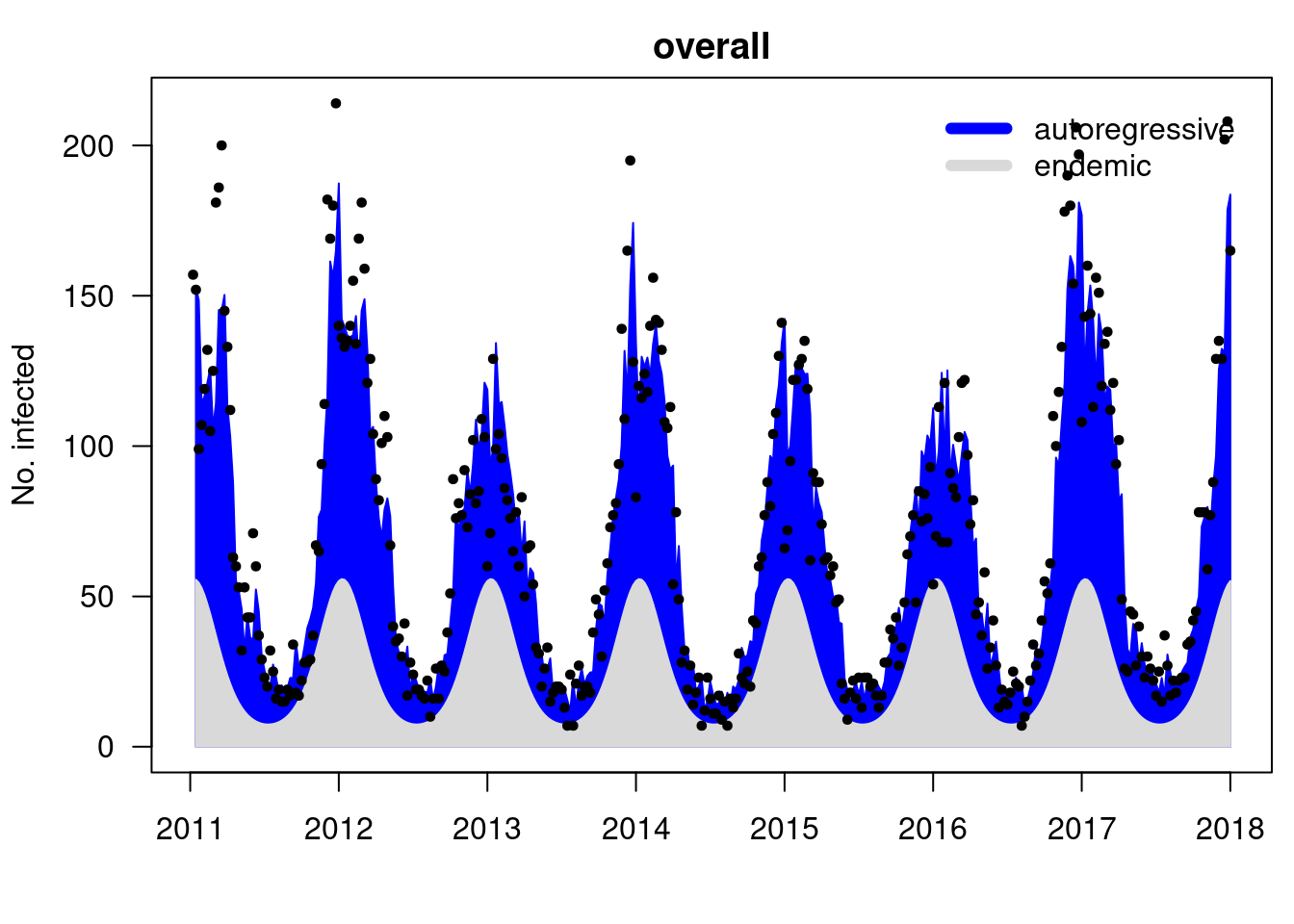
List of 1
 $ overall: num [1:363, 1:8] 153 148 114 117 121 ...
  ..- attr(*, "dimnames")=List of 2
  .. ..$ : NULL
.. ..$ : chr [1:8] "mean" "epidemic" "endemic" "epi.own" ...[1] 0.6210123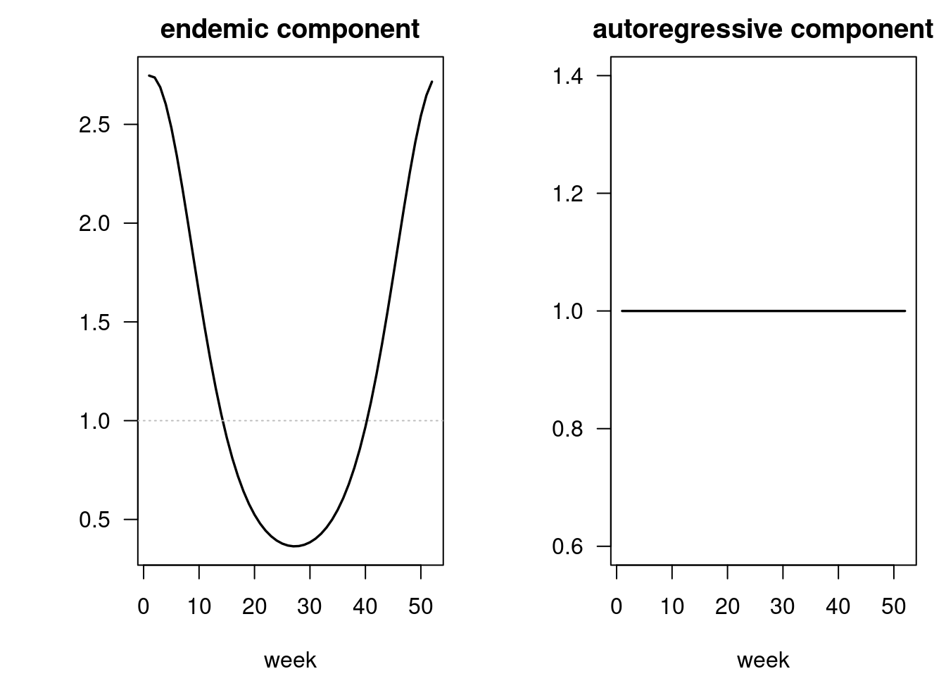
## PIT plot to check model calibration
opar <- par(mfrow = c(1,2))
pit(fit01); title(main = "constant lambda")
pit(fit11); title(main = "seasonal lambda")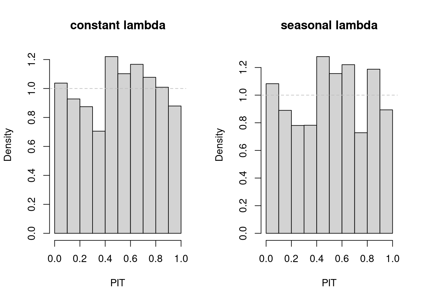
par(opar)
## no clear preference

## check residual correlation
opar <- par(mfrow = c(1,3))
acf(residuals(fit_endemic), main = "endemic-only") # strong residual correlation
acf(residuals(fit01), main = "constant lambda")
acf(residuals(fit11), main = "seasonal lambda")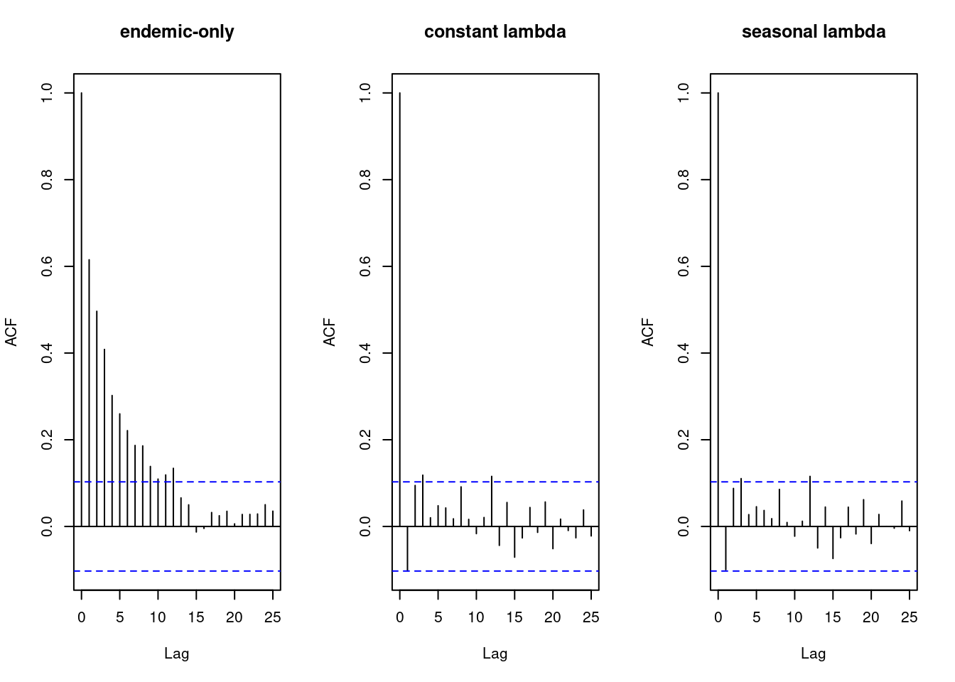
Forecasting
Task
Use oneStepAhead() to produce “rolling” weekly
forecasts, e.g., over the last two years, and plot() the
result. You should also look at a pit() histogram of these
probabilistic forecasts.
Solution
## compute "rolling" weekly forecasts starting from 2016
startidx <- match(2016, year(noro))
osa01 <- oneStepAhead(fit01, startidx, verbose = FALSE)
plot(osa01)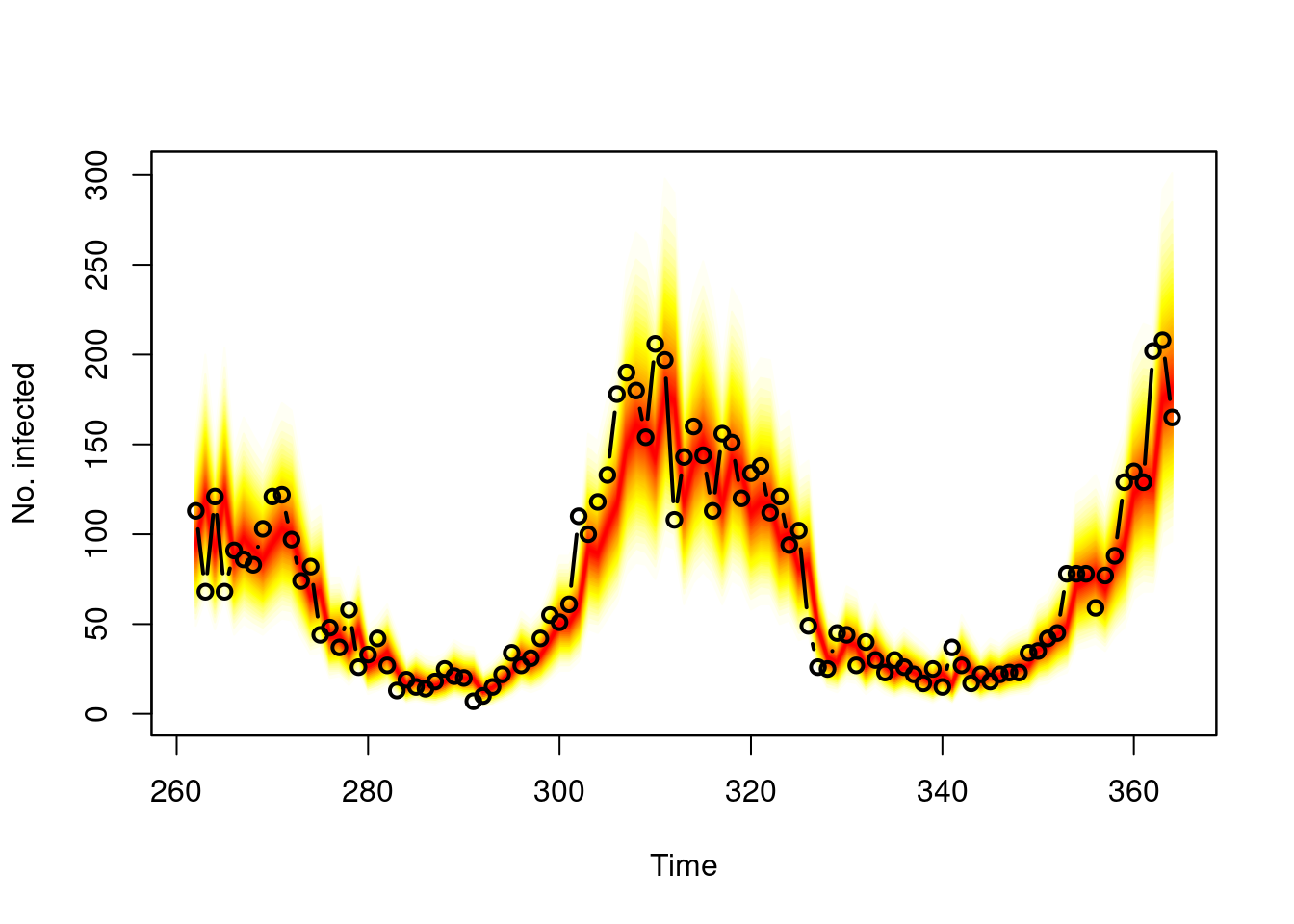
    2.5 % 10.0 % 50.0 % 90.0 % 97.5 %
262    55     67     94    127    147
263    71     86    120    161    186
264    53     64     91    123    142
265    71     87    122    164    189
266    50     61     87    118    137
267    56     69     98    132    153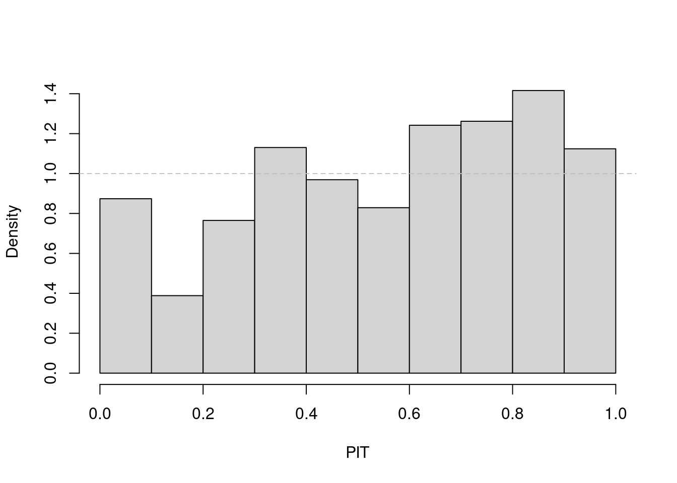
## forecast from fit11 and compare mean scores() (where smaller is better)
osa11 <- oneStepAhead(fit11, startidx, verbose = FALSE)
rbind("constant lambda" = colMeans(scores(osa01)),
      "seasonal lambda" = colMeans(scores(osa11)))
logs rps dss ses
constant lambda 4.169023 10.59943 6.514457 455.2519
seasonal lambda 4.167993 10.56779 6.517539 457.9010